11.3.14 Quasar Classifier (QSOC)
Author(s): Ludovic Delchambre
Goal
The Quasar Classifier (QSOC) module aim to determine the redshift, , of the sources that are classified as quasars by the DSC module (see Section 11.3.2 for more details).
Inputs
The determination of the redshift by QSOC is based on
-
1.
the internally calibrated BP/RP spectra as sampled by SMSgen (see Section 11.3.1)
-
2.
the DSC Combmod probability for the selection of the sources to be processed, namely those having classprob_dsc_combmod_quasar .
-
3.
BP/RP rest-frame quasar templates coming from the weighted principal component analysis (Delchambre 2015) of continuum-subtracted spectra of quasars from the twelfth data release of the Sloan Digital Sky Survey Quasar Catalog (Pâris et al. 2017, hereafter DR12Q) and simulated through the BP/RP simulator (see Section 11.2.3). See Delchambre et al. (2023) for more details on the way these templates were built.
Method
The determination of the redshift of quasars by QSOC is based on the fact that the redshift,
| (11.41) |
turns into a simple offset once considered on a logarithmic wavelength scale
| (11.42) |
where we assume that a given spectral feature standing at rest-frame wavelength is observed at wavelength . Accordingly, given a set of rest-frame templates, , and an observation vector, , that are sampled on the same logarithmic wavelength scale, where is a reference wavelength and is the logarithmic wavelength sampling we use (here or equivalently ), the problem of finding the optimal shift, , between and can be formulated as a minimization problem through
| (11.43) |
where is the uncertainty on and ’s are the coefficients that allow to fit to in a least squares sense while considering a shift that is applied to the templates. The redshift that is associated with the shift being then simply retrieved through . A sub-sampling precision is then obtained by fitting a quadratic curve in the vicinity of the selected shift. For reasons explained in Delchambre (2016) and in Delchambre et al. (2023), we compute a reversed and shifted version of this ,
| (11.44) |
which we refer to as a cross-correlation function (CCF), where is a constant. Figure 11.73 illustrates the CCF of a quasars spectrum from the Sloan Digital Sky Survey (SDSS) against quasar templates coming from Delchambre (2018). Whereas no spectral features can be modelled in shifts associated with local minima, local maxima corresponds to the fit of some of the template emission lines to the observed spectra, while the global maximum usually corresponds to the most probable redshift. As the BP and RP spectra are distinct, we should also note that the effective CCF is actually composed of the sum of two CCF
| (11.45) |
each associated with a given part of the spectrum.
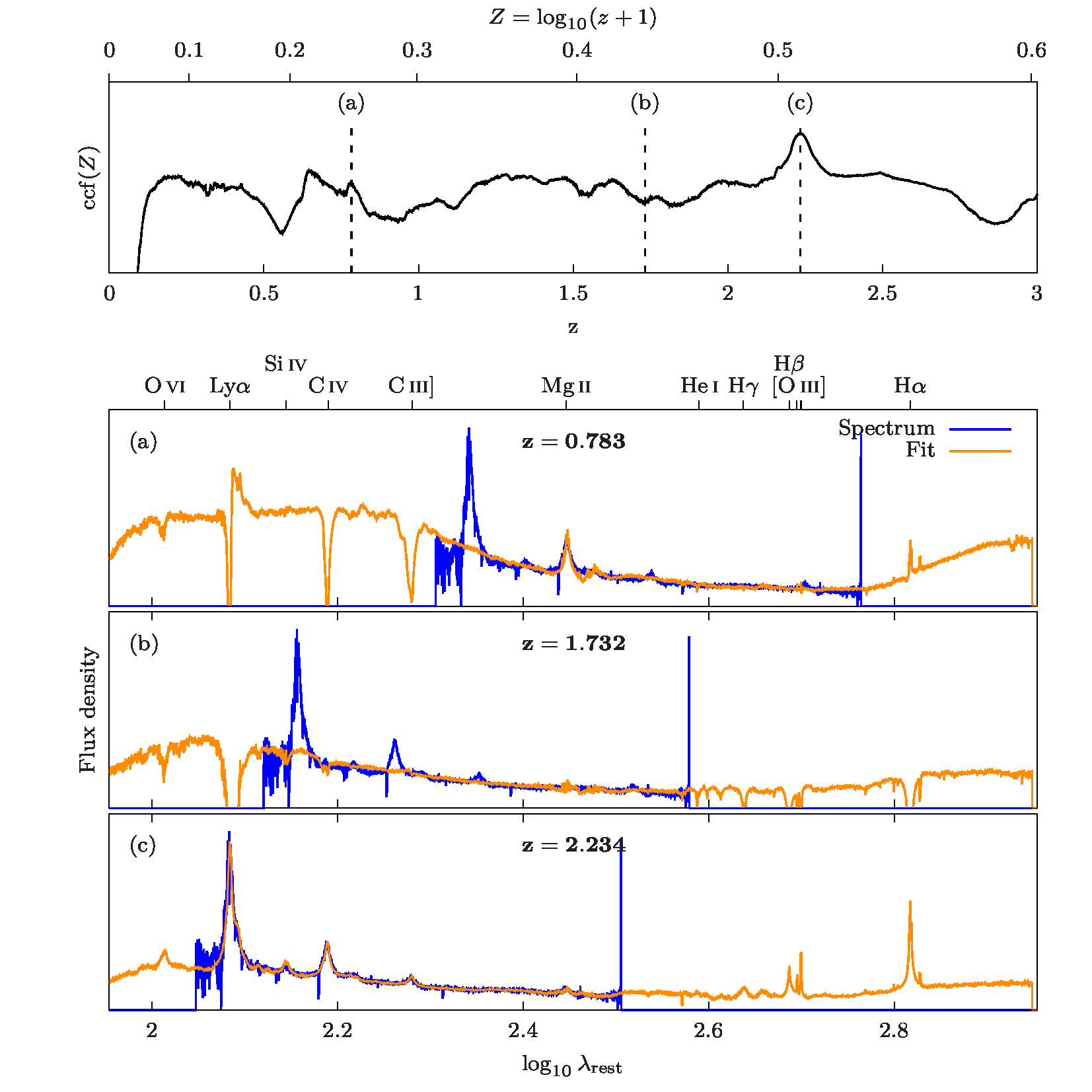
The shift that is selected by QSOC is the one that is associated with the highest score, as defined by
| (11.46) |
where , and (see Delchambre et al. 2023, for details). In this last equation, is the chi-square ratio, ccfratio_qsoc, defined as the value of the CCF evaluated at to the maximum of the CCF,
| (11.47) |
and , zscore_qsoc, is an indicator of the presence of quasar emission lines. A close to one indicates that all the emission lines that we expect at redshift are found in the spectra while the miss of a single emission line often leads to a very low (see Delchambre et al. 2023, for details). In order to facilitate the filtering of the potentially erroneous redshifts by the final user, we further define a binary processing flag, flags_qsoc which is based on these quality indicators as well as on the number of spectral transits and magnitude of the source.
Finally, the redshift that is reported by QSOC is distributed as a log-normal distribution of mean and variance such that its lower and upper confidence intervals, respectively taken as its and quantiles, are given by
| (11.48) |
More information on the QSOC method and on the computation of the can be found in Delchambre et al. (2023).
Outputs
The output of the QSOC module can be found in the following fields of the Gaia qso_candidates table:
-
1.
redshift_qsoc: The quasar redshift, , from Equation 11.41
-
2.
redshift_qsoc_lower and redshift_qsoc_upper: The lower and upper confidence intervals, and , corresponding to the 16% and 84% quantiles of , respectively, as given by Equation 11.48
-
3.
ccfratio_qsoc: The chi-square ratio, , from Equation 11.47
-
4.
zscore_qsoc: The from Equation 11.46
-
5.
flags_qsoc: The QSOC processing flags, .
Scope
QSOC produces redshift predictions in the Gaia qso_candidates table only for sources with a DSC Combmod probability, classprob_dsc_combmod_quasar , while having
-
•
flags_qsoc 16, meaning that the BP/RP spectra are considered as reliable (i.e. flag
Z_BADSPECis not set such that flags_qsoc 16) or the processing of this source rises no warning flag even though the spectrum was considered unreliable (i.e. flags_qsoc = 16). -
•
flags_qsoc 16 but added by other contributors to the Gaia QSO table, as indicated in the source_selection_flags field of the qso_candidates table.
Results
Scope
We provide here a summary of the QSOC performances. We however refer the user to Delchambre et al. (2023) for a more detailed analysis of these results. QSOC performances are assessed by comparing the predicted reshifts against values from the literature. For this purpose, we cross-matched 6,375,063 sources having redshift estimates from QSOC with 790,776 quasars having spectroscopically confirmed redshifts in the Milliquas 7.2 catalogue of Flesch (2021) (i.e. type = 'Q' in Milliquas). The 1 search radius we used then allows us to extract 439 127 QSOC sources with literature redshifts. We should however stress out that neither these redshifts, nor the magnitudes of the cross-matched sources follow realistic distributions, as they inherit from the selection/observational biases that are present in both the Milliquas catalogue and in Gaia. Accordingly, the numbers reported here should be taken with the caution they deserve. That being said, a straight comparison of these predictions shows that of the sources have an absolute error on the predicted redshift, that is lower than 0.1 while this ratio rises to if only flags_qsoc = 0 sources are considered.
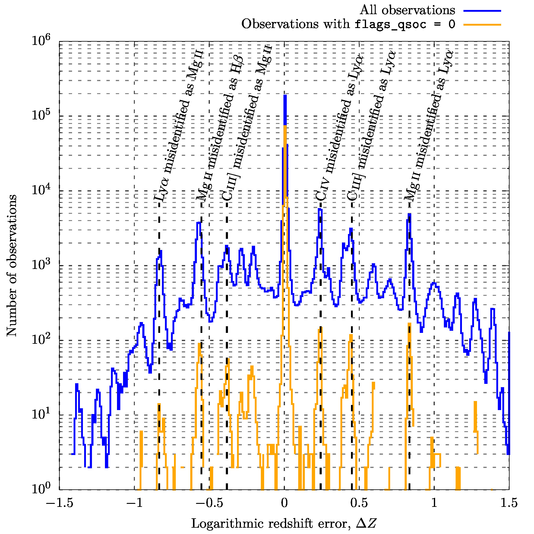
In Figure 11.74, we show the distribution of the logarithmic redshift error, between QSOC redshift, and literature redshift, , for the 439,127 sources we previously identified. The distribution of this logarithmic redshift error provides, in addition to the number of good predictions, a straight visualisation of the mismatches existing between common quasars emission lines. We can see that most of the predictions have and are accordingly in good agreement with their literature values. The emission line mismatches mainly occur with respect to two specific emission lines: C iii] and Mg ii, while the most frequent mismatch occurs when the C iv emission line is misidentified as the Ly emission line, for reasons explained in Delchambre et al. (2023). By requiring that flags_qsoc = 0, we can mitigate the effect of these emission line mismatches without affecting too much the central peak of correct predictions.
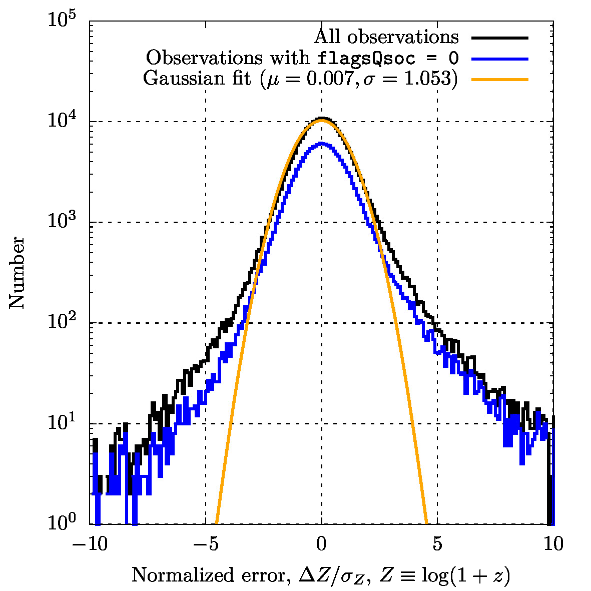
Considering now only predictions, so as to isolate the central peak from Figure 11.74, and computing the normalized logarithmic error as where , we can see that the distribution of approximately follows a Gaussian distribution of median 0.00744 and standard deviation – extrapolated from the inter-quartile range – of ( if flags_qsoc = 0 observations are considered). The normality of is expected from Section 11.3.14, though large tails are present that come from systematics and from a smooth background of random predictions associated with very low signal-to-noise ratio (SNR) observations.
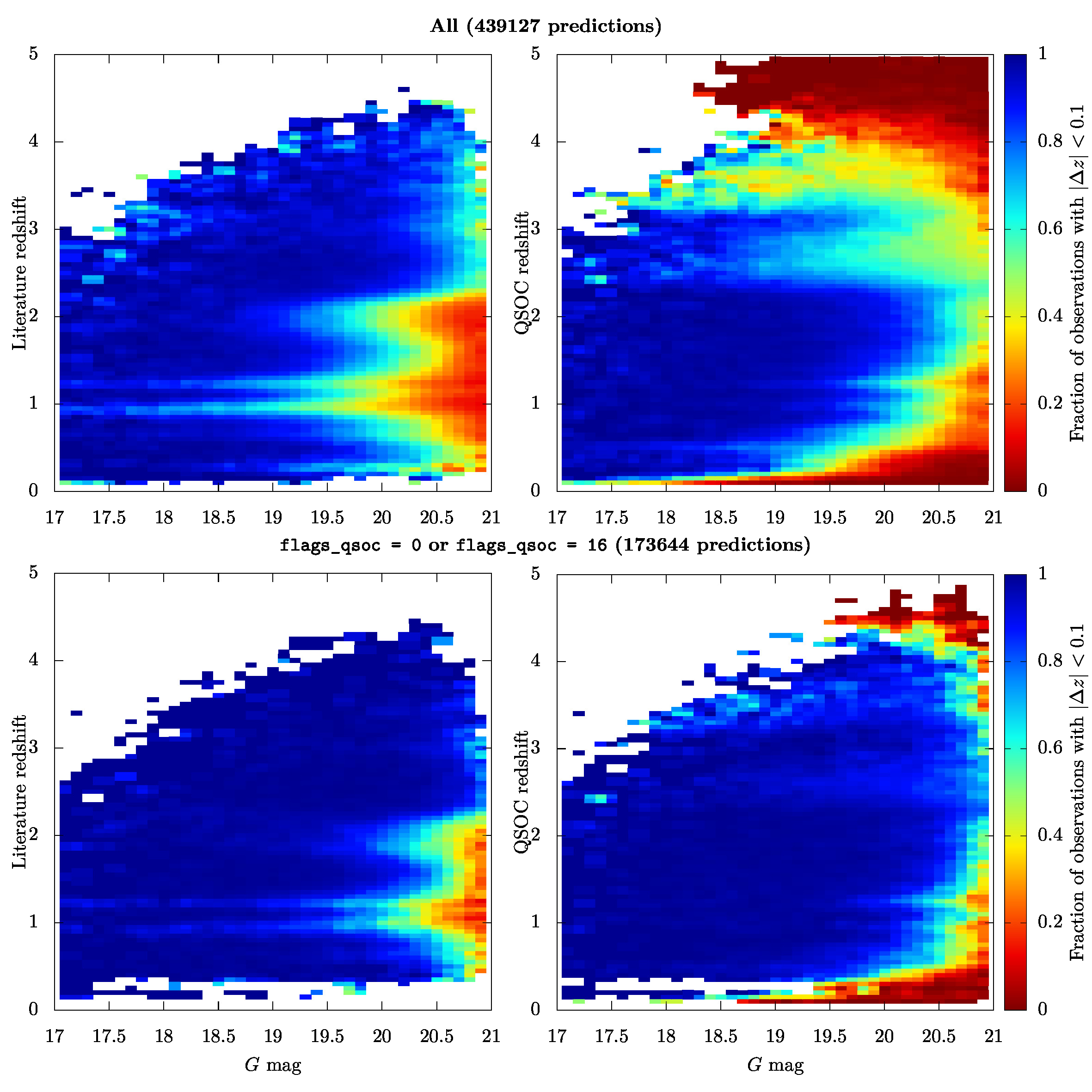
Finally, in Figure 11.76, we plot the fraction of sources with with respect to literature/QSOC redshift and Gaia magnitude for all the 439,127 predictions found in the Milliquas catalogue and for those where we encounter no processing issues (i.e. flags_qsoc values – are not set, such that flags_qsoc or flags_qsoc ). This plot can be regarded as a way to evaluate the purity/completeness of the QSOC predictions as it straightly provides the fraction of observations in terms of predicted redshift (i.e. purity) and in terms of ‘true’ redshift, assimilated here to be the literature redshift (i.e. completeness). We can note an overall decrease of the performances as we go to fainter objects. This is an obvious consequence of the generally lower SNR of these objects. Regarding the QSOC completeness (left part of Figure 11.76), we can note two problematic regions in and around that are due to the fact that only the Mg ii emission line is covered in the BP/RP spectra of quasars and to the misidentification of the C iv emission line as Ly in quasars, as explained in Delchambre et al. (2023). The lower purity seen in quasars having QSOC redshift or , comes from the rarity of these very low/high redfshift quasars such that any false predictions towards these loosely populated regions are largely reflected in the final fraction of observations. Again, appropriate cuts on the flags_qsoc allow to circumscribe these wrong predictions to limited regions of the magnitude/redshift space, as seen by comparing the lower and upper panels of Figure 11.76.
Use
A few points of attention should be kept in mind while using QSOC predictions:
-
•
The set of sources processed by QSOC aim to be complete rather than pure (i.e. we voluntarily set a very low threshold on the DSC Combmod probability of classprob_dsc_combmod_quasar ). As a consequence, we expect most of our processed sources to be stellar contaminants rather than genuine quasars such that users interested in purer samples should consider using stricter selection rules as classlabel_dsc_joint 'quasar' or those described in (Gaia Collaboration et al. 2023b, Section 8).
-
•
QSOC is –by construction– designed to process Type-I/core-dominated quasars with broad emission lines in the optical and accordingly yield only poor predictions on galaxies, type-II AGN and BL Lacertae/Blazars objects, that would in any case have flags_qsoc .
-
•
The presence of the sole Mg ii emission line in the observed BP/RP spectra of quasars at can lead to a higher rate of degeneracy between redshifts in this particular range. Also, the mismatch between the C iv and Ly emission lines in quasars is a frequent case of misidentification. These degeneracies being more frequent amongst faint sources.
-
•
Because SMSGen, described in Section 11.3.1, do not provide covariance matrices on the integrated flux (see Creevey et al. 2023), the computed , from Equation 11.43, is systematically underestimated and is consequently not published in Gaia DR3. The computed redshift and associated confidence intervals, and from Equation 11.48, though appropriately re-scaled, might sporadically suffer from this limitation.
-
•
Requiring that flags_qsoc may lead to a large amount of predictions that are discarded, especially at faint magnitudes. For users interested in mag quasars, we hence suggest to use a less stringent cut of the form flags_qsoc or flags_qsoc , where we encounter no processing issue (i.e. flags – are not set) even when the BP/RP spectra are unreliable (i.e. flag can be set).