11.3.4 General Stellar Parametrizer from Spectroscopy (GSP-Spec)

GSP-Spec (Recio-Blanco et al. 2023) estimates the stellar atmospheric parameters, individual chemical abundances and Diffuse Interstellar Band (DIB) parameters from combined RVS spectra of single stars. No additional information (astrometric, photometric or BP/RP data) is considered, allowing a purely spectroscopic treatment. Two different algorithms described in Recio-Blanco et al. (2016), MatisseGauguin and ANN, are applied for atmospheric-parameter estimation. Individual abundances and DIB parameters are only estimated from the MatisseGauguin atmospheric parameters, using the Gauguin algorithm (Recio-Blanco et al. 2006) and Gaussian fitting methods (Zhao et al. 2021), respectively. Uncertainties are estimated from 50 Monte Carlo realisations considering the spectral flux uncertainties per pixel provided by CU6. For each realisation, a new complete parameterisation, from atmospheric parameters to related chemical abundances and DIB parameters, is performed. Upper and lower confidence values are provided from quantiles 84th and 16th, respectively.

GSP-Spec uses as input combined RVS spectra and their flux uncertainties per pixel. The spectra are continuum normalised from CU6 pipelines, however, GSP-Spec reviews the continuum placement during the spectra parameterisation procedure. In addition, the spectra are rebinned from 2400 pixels to 800 pixels (without reducing the spectral resolution thanks to the RVS oversampling), allowing to increase their signal-to-noise (SNR) ratio. The RVS spectra analysed by GSPspec during DR3 operations were selected to have SNR$>$20 before resampling.

Further input data are model grids of synthetic RVS spectra. The spectra have been derived from MARCS atmospheric models of FGKM-type stars (Gustafsson et al. 2008), using the TURBOSPECTRUM spectral synthesis code (Plez 2012). The associated line lists are those of Contursi et al. (2021). These models are used for the stellar atmospheric parameters ($T_{\mathrm{eff}}$, $\log g$, $[\mathrm{M}/\mathrm{H}]$ and [$\alpha$/Fe]), but also for the individual abundances estimate, for which a fifth dimension is added on [X/Fe], with X being the considered chemical element. We used an empirical law for the microturbulence parameter. This parametrized relation is a function of $T_{\mathrm{eff}}$, $\log g$ and $[\mathrm{M}/\mathrm{H}]$, and has been derived from $V_{\mathrm{micro}}$ literature values for the Gaia-ESO Survey (Bergemann et al., in preparation).

Two main procedures are implemented in GSP-Spec: MatisseGauguin (results published in the table astrophysical_parameters) and ANN (published in the astrophysical_parameters_supp table). Please refer to Recio-Blanco et al. (2023) for a detailed description of the methodology.

The MatisseGauguin parameterisation procedure, producing the GSP-Spec atmospheric parameters, individual chemical abundances and DIB parameters included in the astrophysical_parameters table, is as follows:

1. 1.

   Stellar parameters initialization with DEGAS: Once the RVS spectra are rebinned to 800 pixels, the DEGAS decision tree method (Kordopatis et al. 2011), considering the entire parameter space of the grid (FGKM-type stars), is used to derive a first guess in $T_{\mathrm{eff}}$, $\log g$, $[\mathrm{M}/\mathrm{H}]$ and [$\alpha$/Fe].

2. 2.

   Matisse algorithm application: The MATISSE algorithm (Recio-Blanco et al. 2006) is applied following an iterative procedure in the parameter estimation to overcome non-linearity problems. MATISSE is a projection method in the sense that the full input spectra are projected into a set of vectors derived during a learning phase, based on the noise-free reference grids. The noise optimization is taken into account thanks to a Landweber algorithm during the covariance matrix inversion and it is adapted to each application. These vectors are a linear combination of reference spectra and could be viewed roughly as the derivatives of these spectra with respect to the different stellar parameters. MATISSE is, thus, a local multi-linear regression method. The MATISSE projection is first applied around the DEGAS solution in a local environment of $\pm$500 K in $T_{\mathrm{eff}}$, $\pm$0.5 dex in $\log g$, $\pm$0.25 dex in $[\mathrm{M}/\mathrm{H}]$ and $\pm$0.20 dex in [$\alpha$/Fe]. This produces a second solution around which MATISSE is applied again. This iterative procedure is repeated until convergence, within a maximum of 10 iterations.

3. 3.

   Refinement of parameters with GAUGUIN: The GAUGUIN algorithm is applied around the final MATISSE solution of the previous step, considering a local environment of $\pm$250 K in $T_{\mathrm{eff}}$, $\pm$0.5 dex in $\log g$, $\pm$0.25 dex in $[\mathrm{M}/\mathrm{H}]$ and $\pm$0.20 dex in [$\alpha$/Fe]. GAUGUIN (Bijaoui et al. 2012; Recio-Blanco et al. 2016) is a classical, local optimization method implementing a Gauss-Newton algorithm. It is based on a local linearization around a given set of parameters that are associated with a reference synthetic spectrum (via linear interpolation of the derivatives). Its goal is to find the direction in the parameter space that has the highest negative gradient as a function of the distance. Once this direction is found, the method proceeds in an iterative way, by modifying the initial guess of the studied parameter and re-calculating the gradient again, until convergence of the parameter solution. A few iterations are carried out through linearization around the new solutions, until the algorithm converges towards the minimum distance. In practice, and to avoid trapping into secondary minima, GAUGUIN is initialized by parameters independently determined by other algorithms such as MATISSE. The final MATISSE+GAUGUIN solution in $T_{\mathrm{eff}}$, $\log g$, $[\mathrm{M}/\mathrm{H}]$ and [$\alpha$/Fe] is considered in the following.

4. 4.

   Continuum placement and spectra normalization: The parameters solution of the previous step is used to re-estimate the continuum placement. This step is particularly important in the case of cool stars, having pseudo-continuum flux values lower than one. The continuum placement and normalization procedure is described in detail in Santos-Peral et al. (2020). In this step, the spectrum flux is normalised over the entire RVS wavelength domain. To this purpose, the observed spectrum (O) is compared to an interpolated synthetic one (S) with the same atmospheric parameters. First, the most appropriate pixels of the residual (R = S/O) are selected using an iterative procedure implementing a linear fit to R followed by a $\sigma -$clipping. Then, the residual trend is fitted with a low degree polynomial. Finally, the normalised spectrum is obtained after dividing the observed spectrum by a linear function resulting by the fit of the residual.

5. 5.

   Iteration in the atmospheric parameters solution following the continuum refinement: The module comes back to step 1, to re-estimate the atmospheric parameters using the new spectra normalization. This loop is performed five times, iterating on the parameters and the continuum placement. The final parameters solution in $T_{\mathrm{eff}}$, $\log g$, $[\mathrm{M}/\mathrm{H}]$ and [$\alpha$/Fe] is saved in the memory, as well as the final normalized spectrum. A goodness-of-fit (g.o.f.) between the observed and the synthetic spectrum interpolated to the final atmospheric parameters is derived and saved. This g.o.f. is reported in the final table only for the original observed spectra, not including Monte Carlo variations of the flux (see step 8).

6. 6.

   Chemical abundances per spectral line using GAUGUIN: Considering the final atmospheric parameters solution and normalized spectrum, selected spectral lines are considered for individual chemical abundance estimates. For each line identified in the list, a specific reference synthetic spectra grid is interpolated at the input atmospheric parameters in order to measure the abundance from the related chemical element responsible for the line absorption. This grid now includes a large range in the element abundance dimension (AX). First of all, a local normalization around the line is performed (Santos-Peral et al. 2020). A minimum quadratic distance is then calculated between the reference grid and the observed spectrum, providing a first guess of the abundance estimate (A0). This first guess is optimised via the GAUGUIN algorithm, carrying out iterations through linearisation around the new solutions. The algorithm stops when the relative difference between two consecutive iterations is less than a given value (typically one hundredth of the grid abundance step).

7. 7.

   Diffuse Interstellar Band parameters: After a specific local normalisation around the DIB feature at 862 nm, the DIB parameters are extracted (Zhao et al. 2021). More particularly, the DIB characteristics are derived from the spectra of late-type stars by subtracting the corresponding synthetic spectra. For early-type stars we applied a specific model based on the Gaussian process that needs no prior knowledge of the stellar parameters.

8. 8.

   CN over/under abundance proxy: a cyanogen line is analysed subtracting the corresponding synthetic spectra and estimated the equivalent width of the remaining feature (the value is positive for a CN over-abundance or negative for a CN under-abundance with respect to the standard value of [CN/Fe]=0.0 dex. To this purpose, the same Gaussian fitting procedure employed for DIB parameters of late-type stars is used, although allowing negative equivalent width values for CN under abundances.

9. 9.

   Monte Carlo iterations using flux uncertainties: flux uncertainties provided by CU6 are used to estimate the uncertainties in the GSP-Spec output parameters. To this purpose, 50 Monte Carlo realizations of the spectral flux are implemented. Variations of the spectral flux per pixel are generated, following a Gaussian distribution whose standard deviation is equal to the input flux uncertainties. For each realisation, a new complete parameterisation is performed, starting from step 1. This allows final set of 50 values for each atmospheric parameter, each spectral-line abundance and each DIB fitting parameter. Thanks to this, median, upper and lower confidence values are provided from quantiles 50th, 84th and 16th, respectively.

10. 10.

    Individual chemical abundances per element: The final chemical abundances per element are derived by combining the independent abundance estimates of all the lines of the same element. To this purpose, a weighted mean is calculated, using the inverse of the line-abundance uncertainty (defined as the upper minus lower abundance value of all the MC realisations of that line abundance) as a weight.

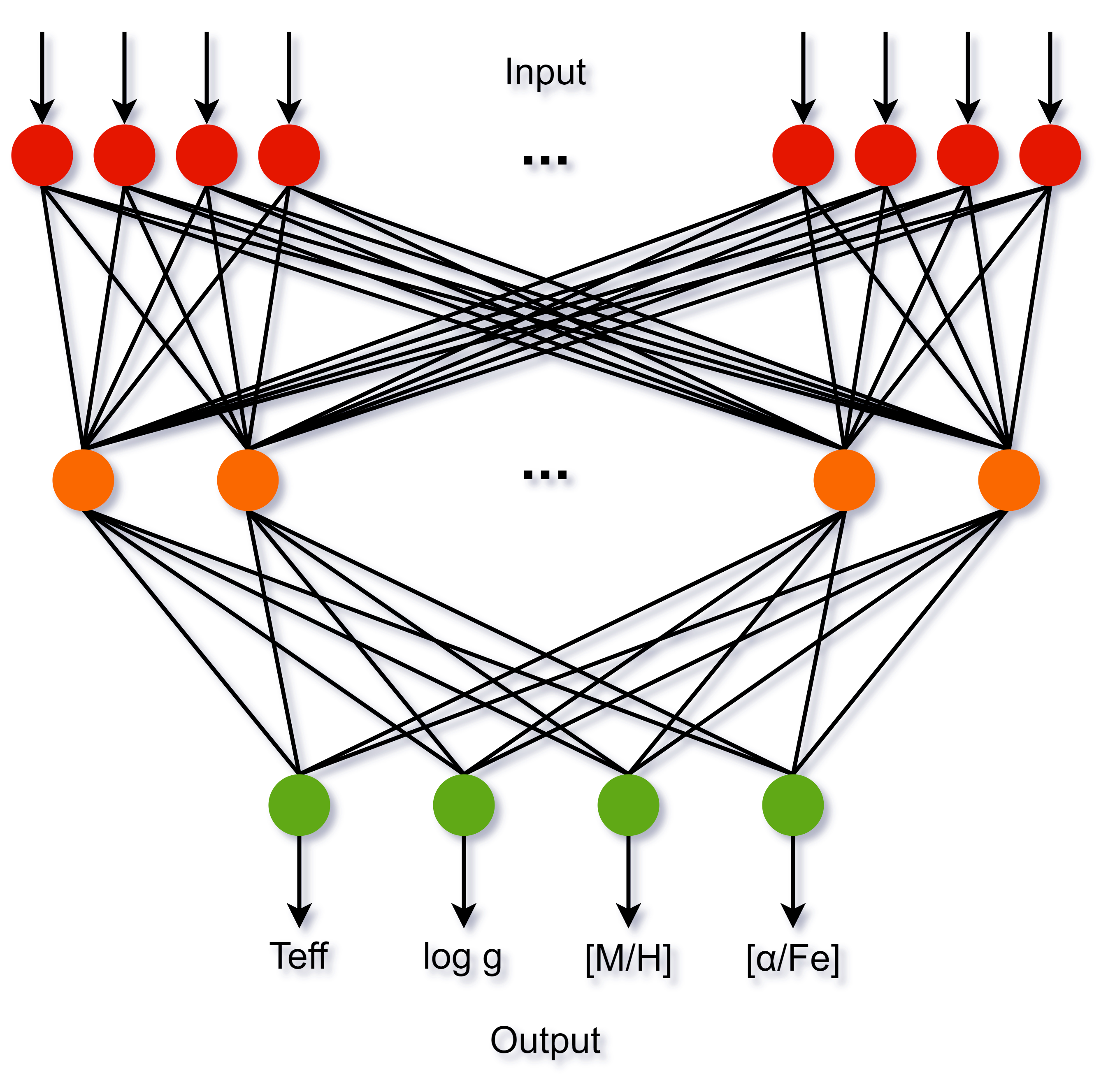
The Artificial Neural Network (ANN) parameterisation procedure is responsible for the GSP-Spec atmospheric parameters published on the astrophysical_parameters_supp table. The architecture used for ANN is feed-forward with three fully connected layers, see Figure 11.22. The input layer has as many neurons as predictor variables and the output layer has as many neurons as variables to be predicted. In this case, the input layer corresponds to the pixels in the spectrum (800) and the output layer to the four APs. The hidden layer connect both input and output layers and the number of neurons has been determined empirically between 50 and 100 for nets trained with low to high SNR spectra, respectively. The ANN analysis procedure is as follows:

1. 1.

   ANN selection: ANN behaves well in the presence of noise (Manteiga et al. 2010), proving that it is a robust method when performing the estimation of APs. However, the error in the estimates depends on the signal to noise ratio (SNR) so, in order to reduce the error in the estimation, we decided to discriminate between five SNR ranges, see Table 11.21, training a network for each range. For each spectrum we use the SNR value, given by CU6, to select which net performs the parameter estimation.

2. 2.

   Check boundaries: Some RVS spectra have NaN values at the beginning or at the end of the spectrum, caused by radial velocity corrections, that could lead to a heavy variation in flux. This can be interpreted as an important characteristic by the ANN, and to avoid this behaviour, we truncate these zero values to the mean of the spectrum.

3. 3.

   Normalisation: A min-max normalisation procedure is applied to the RVS spectra (800 pixels) to avoid geometric biases, and to ensure that all dimensions of the spectrum are in the same range to have the same importance in training.

4. 4.

   Parameter estimation: Once the net has been selected, it is fed with the normalised spectrum deriving the estimations of $T_{\mathrm{eff}}$, $\log g$, $[\mathrm{M}/\mathrm{H}]$ and [$\alpha$/Fe]. These parameters are also normalised so, a de-normalisation procedure is applied to return the correct values.

5. 5.

   Monte Carlo iterations using flux uncertainties: The same procedure used for MatisseGauguin (see item 9 above) is also applied for ANN, obtaining the median, upper and lower confidence values from quantiles 50th, 84th and 16th, respectively.

The activation function used for input and output layers is lineal, but for the hidden layer the logistic function is the chosen one.

The learning function used to train ANNs is the back-propagation algorithm, that can be interpreted as a problem of minimization of the error existing between the obtained and desired outputs.

In order to select the ANN that best generalizes avoiding the overtraining, we use the early stopping procedure, obtaining the net that minimize the error by stopping the training at the point when performance starts to degrade. We also initialize weights in the range [-0.2,0.2].

The learning rate, used to determine the speed and quality of learning, has been determined empirically in the range [0.001, 0.2].

Due to the fact that the effectiveness of the ANN depends on the input ordering, we perform ten trains with different initializations, selecting the one with minimum error. Each train has a limit of one thousand iterations because we observed that beyond that number, the training process does not improve but the computational cost increases.

To train ANNs we use the grid of synthetic spectra mentioned before (Section 11.3.4), since there is no noise model of Gaia RVS, we empirically determined the relation between the noise given by CU6 and the Gaussian noise that we have to use to train the nets, as it is shown in Table 11.21

To guarantee that all inputs are in a comparable range, all spectra used to train ANNs must be normalized with the same procedure. Desired parameters ($T_{\mathrm{eff}}$, $\log g$, $[\mathrm{M}/\mathrm{H}]$ and [$\alpha$/Fe]) are also normalized in order to have the same importance in the training process. In this case, the normalization is performed using the maximum and minimum values of the grid.

As a result, we obtained five trained nets to estimate the atmospheric parameters according to these SNR ranges. Each network estimates the parameters of a given spectrum according to the signal to noise ratio provided by CU6.

MatisseGauguin results provide 23 independent APs in the astrophysical_parameters table. This includes: $T_{\mathrm{eff}}$, log g, $[\mathrm{M}/\mathrm{H}]$, [$\alpha$/Fe], goodness-of-fit over the entire spectral range, individual chemical abundances of [N/Fe], [Mg/Fe], [Si/Fe], [S/Fe], [Ca/Fe], [Ti/Fe], [Cr/Fe], [Fe/M], [FeII/M], [Ni/Fe], [Zr/Fe], [Ce/Fe], [Nd/Fe], CN equivalent width and its fitting parameters, DIB equivalent width and its fitting parameters. In addition, for each atmospheric parameter, chemical abundance and equivalent width, upper and lower confidence values are provided. For each chemical element abundance, the number of used spectral lines, as well as the line-to-line scatter are presented.

ANN results provide 4 APs in the astrophysical_parameters_supp table. This includes: $T_{\mathrm{eff}}$, $\log g$, $[\mathrm{M}/\mathrm{H}]$, [$\alpha$/Fe] and their upper and lower confidence values and a goodness-of-fit over the entire spectral range.

Finally, following the results of the internal GSPspec validation, a GSPspec catalogue flag has been implemented during the post-processing and published in both the astrophysical_parameters and the astrophysical_parameters_supp tables. The GSPspec catalogue flag is a chain of 41 characters including all the adopted failure criteria and uncertainty sources considered during the post-processing. In this chain, value “0” is the best, and “9” is the worse, generally implying the parameter masking. The order of the individual flags is listed in Table 11.22, including the possible adopted values for each of them. Please refer to Recio-Blanco et al. (2023) for a detailed description of the GSPspec catalogue flags.

All results are provided for stars with SNR$>$20 (for an estimate of the RVS signal-to-noise see the expected$\mathrm{\_}$sig$\mathrm{\_}$to$\mathrm{\_}$noise field). During the post-processing, dubious results were filtered out based on processing flags. In particular, results out of the validity range of the reference synthetic spectra grids (essentially FGK-type stars) are flagged thanks to the extrapolation character of the GSP-Spec catalogue flag chain.

A detailed description of GSP-Spec results, including an in depth analysis of methodological biases and comparison with literature parameters can be found in Recio-Blanco et al. (2023). Gaia self-consistent calibrations are proposed for the observed biases. It is important to underline the fact that the use of GSP-Spec catalogue flags is crucial for any scientific use of the GSP-Spec results.

ANN shows no important internal bias as inferred from tests with synthetic spectra, see Table 11.23. However, compared to the literature, ANN results present important biases that have to be taken into account, see Table 11.24.

In Figure 11.23 the parameterisation for all stars (5 524 387) is shown, considering all possible flag values.

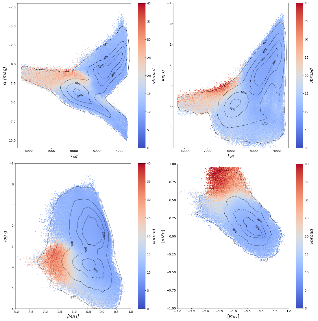
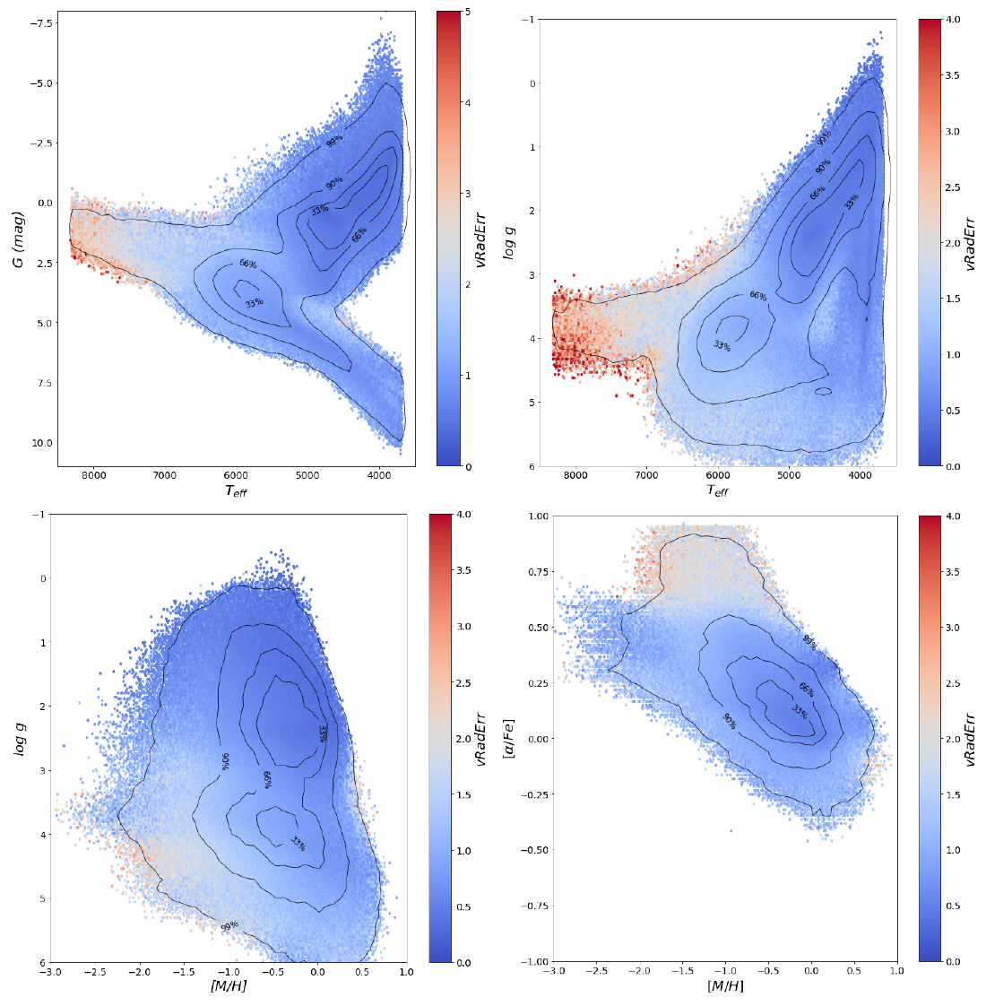
Plots in Figure 11.24 and Figure 11.25 show that the stars with vbroad values greater than 20 km/s, or radial velocity errors greater than 2 km/s, occupy specific regions of the parameter space, mostly coincident for both.

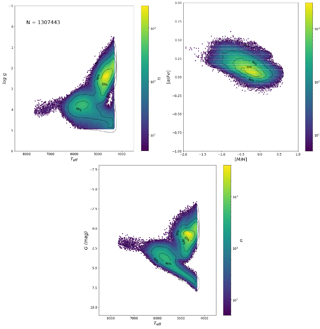
In Figure 11.26 only the best quality parameterisations are shown (1 307 443), this means stars with no bias induced by vbroad nor radial velocity, also stars with noise uncertainties flag equals to 0 and parameters without extrapolations.