11.3.13 Unresolved Galaxy Classifier (UGC)
Author(s): Ioannis Bellas-Velidis, Despina Hatzidimitriou
Goal
The Unresolved Galaxy Classifier (UGC) module aims to estimate the redshift of unresolved galaxies observed by Gaia. The module processes every source that is classified as ”galaxy” by the DSC (Section 11.3.2) with a probability above a predefined threshold and with a magnitude within a specific range. UGC predicts the redshift of the source by applying to its BP/RP spectrum a supervised learning model based on Support Vector Machines (SVM, (Cortes and Vapnik 1995)). Two other SVM models are used to validate the estimated redshifts. The SVMs are trained on a set of Gaia spectra of sources with redshifts provided by an external catalogue (see Section 11.3.13). The module defines the eligibility of the predicted redshift for inclusion in the publishable output, by applying a set of rules to the validation results for particular source parameters (see Section 11.3.13).
Inputs
The determination of the redshift of a source is based on
-
•
the internally calibrated BP/RP mean spectrum as sampled by SMSgen (see Section 11.3.1);
-
•
the DSC Combmod probability for a source to be a galaxy, classprob_dsc_combmod_galaxy, which is used in the selection of the sources that will be processed;
-
•
the mean magnitude, phot_g_mean_mag, and the mean magnitudes in the BP phot_bp_mean_mag and in the RP band phot_rp_mean_mag; the is used for source selection, while all are used for the derivation of the eligibility of the resulting redshifts for inclusion in the publishable output;
- •
-
•
the three SVM models (see Section 11.3.13), which are used for the redshift prediction and validation.
SVM models
The three SVM models are prepared in advance by a dedicated module, UGC_Learn. The module, which is not part of the Apsis chain, is executed locally. The trained models are exported as files and can be imported to the chain. The learning module utilizes the library LIBSVM Chang and Lin (2011) for the SVM model development and provides configuration, tuning, training and testing functions. As a supervised learning method, the SVM requires a training data set for model preparation. Each instance in the set contains one vector of several input features (input variables) and one target value (the desired output). In order to estimate the prediction performance of the trained SVM model, a testing set must be prepared in the same way as the training set.
A common setup has been implemented for the SVM model preparation (see LIBSVM for details):
-
•
The Standardization Unbiased method is selected, to scale the target data and the vector elements to the range (the target is not scaled in the c-SVM).
-
•
The radial basis function (RBF) is chosen as the kernel function to map the training vectors into a higher multidimensional space.
-
•
The tolerance of the termination criterion is set to .
-
•
Shrinking heuristics are used to speed up the training process.
-
•
A four-folded tuning (cross-validation) is applied to determine the optimal kernel parameter and the penalty parameter of the error term in the optimization problem.
In the case of UGC, the instances of the data set are selected Gaia sources (galaxies) with known redshifts. The target value is the redshift of the source (t-SVM) or a specific value derived from it (r-SVM and c-SVM). The elements of the input vector are the integrated flux values of the sampled BP/RP spectrum of the source provided by SMSgen. The edges of the BP spectrum are truncated by removing the first 34 and the last 6 samples, to avoid low S/N data. Similarly, the first 4 and the last 10 samples are removed from the RP spectrum. The “truncated” spectra are then concatenated to form the vector of 186 (80+106) fluxes.
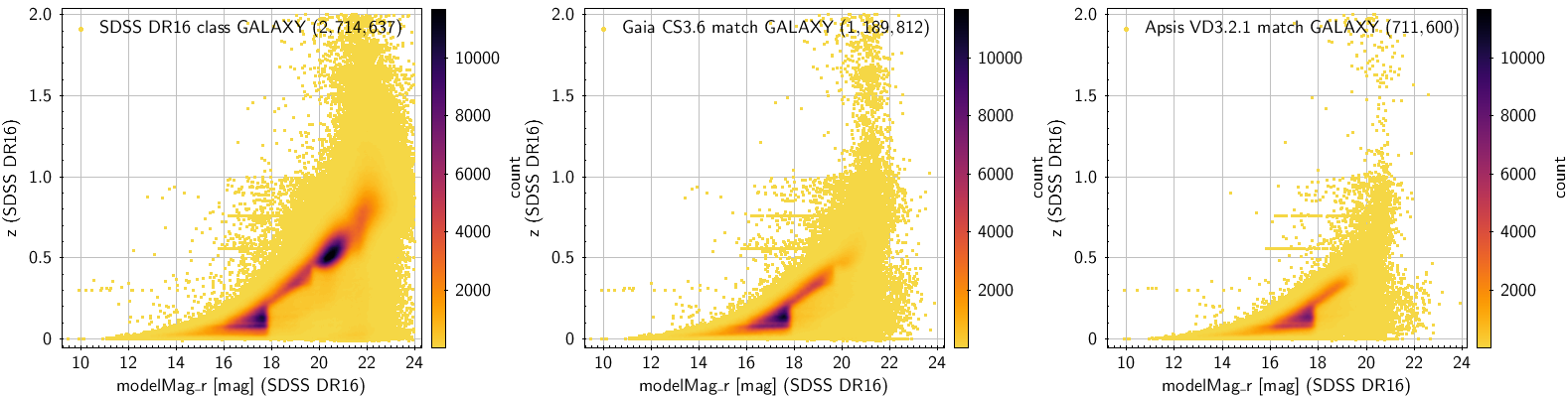
The sources used for the training and the testing sets were selected from the SDSS DR16 archive (Ahumada et al. 2020). We used the SpecObj and PhotoObj tables (SDSS “views”) which provide for each observed extragalactic object, its spectroscopic classification, magnitude in five bands, photometric size (e.g Petrosian radius), spectroscopic redshift, and many of other parameters. There are 2 787 883 objects of SDSS class ”GALAXY” that appear in both tables. We rejected sources with bad or missing photometry, size or redshift, thus reducing the number of galaxies to 2 714 637. The left panel of Figure 11.59 shows the distribution of redshift vs. magnitude for these galaxies. The distribution is far from uniform and displays two main clumps, one at low redshift () and one in the redshift range . This non-uniformity is a known feature of the SDSS spectroscopy of extragalactic sources (see BOSS Target Selection). Despite this, the SDSS survey provides the largest existing database of accurate spectroscopic redshifts of galaxies.
The 2 714 637 SDSS galaxies were cross-matched (using radius 0.54”) with the observed Gaia sources. The result was a table of 1 189 812 SDSS galaxies also observed by Gaia. Due mainly to the photometric limit of the Gaia observations, most of the high-redshift galaxies () are absent from this table and the conspicuous clump in the redshift range has almost disappeared in the magnitude vs redshift distribution (see central panel in Figure 11.59). Of the 1 189 812 galaxies, a sub-sample of 711 600 objects were included in the validation data set and processed by SMSgen during the Apsis validation, thus providing sampled BP/RP spectra for the training and testing sets. The magnitude vs redshift distribution for these objects is shown on the right panel of Figure 11.59). The high redshift regime is very sparsely populated and would lead to a very unbalanced training set. Thus, an upper limit of was imposed to the SDSS redshifts, rendering a total of 709 449 sources with forming a base set.
For the preparation of the training set, a number of conditions have been imposed to sources in the base set: (i) the sources must be brighter than a certain magnitude limit, , in order to avoid spectra of faint sources, (ii) the final BP/RP spectrum must be derived from a minimum of six transits (epochs of observations) and (iii) the mean flux in the truncated blue and red parts of the BP/RP spectrum must lie in the ranges and , respectively, in order to exclude potentially poor quality spectra, (iv) the image size, as characterised in SDSS by the Petrosian radius, must be in the range , in order to exclude suspiciously compact or significantly extended galaxies, (v) interstellar extinction must be below a certain upper limit, (provided by SDSS), to avoid highly reddened sources, and (vi) a lower limit, , is imposed to SDSS redshift in order to exclude nearby extended galaxies. Table 11.33 provides the list of conditions (Col. 1), the total number of spectra that do not fulfill the corresponding condition (Col. 2) and the number of sources (Col. 3) that remain in the set, after the sequential application of each one of these conditions. The final set, referred to as the “clean set”, consists of 377 875 good quality spectra that can be used for SVM training. Of these, 6000 sources were selected randomly in SDSS redshift sub-ranges of size in .
| Source acceptability rule | Rejected sources | Remaining sources |
| Galaxies with (base set) | 709 449 | |
| 306 231 | 404 219 | |
| and | 84 684 | 391 026 |
| and | 4 299 | 390 806 |
| (neither very compact nor very extended) | 18 209 | 378 770 |
| (to exclude sources strongly influenced by extinction) | 947 | 378 288 |
| (to exclude nearby galaxies) | 1 373 | 377 875 |
For the testing set no conditions were imposed. All 703 449 spectra in the base set, not used for training, were included in the testing set. The distribution of sources in redshift bins for the training and the testing sets are shown in Table 11.34. The lack of balance in the training set is obvious in this table, and is caused by the small number of higher redshift galaxies present in the clean set.
| z-range | Total | ||||||
| Training set | 1 600 | 1 600 | 1 100 | 900 | 500 | 300 | 6 000 |
| Testing set | 222 664 | 291 368 | 117 148 | 65 012 | 6 555 | 702 | 703 449 |
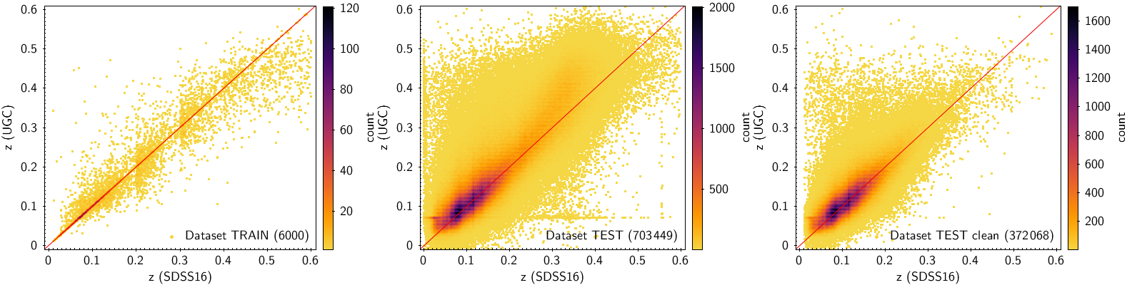
In UGC, the redshifts are estimated by t-SVM, which implements a regression model of the type -SVR of the LIBSVM library, trained for redshifts in the range . The overall performance of the model is given by the mean () and the standard deviation () of the difference between the estimated and the real (target) redshifts for this range . The internal test, i.e. applying t-SVM to the 6000 training data itself, yields and . The external test, which is performed on the 703 449 testing data in the base set not used for training, yields and . These values indicate that the performance is worse in this case, which is expected as this set includes all data, without any filtering. If a clean testing set of 371 875 spectra (after removing the 6000 training data from the clean set) is used, the performance is improved significantly, with and .
The performance varies with redshift. This is a consequence of the lack of balance in the training sample, mentioned above. A comparison of the SVM-estimated and the SDSS redshifts is shown in Figure 11.60 for the internal test (left panel), for the external test using the testing set (middle panel) and for test using the clean testing set (right panel). In the case of the internal test, the SVM underestimates larger redshifts because of the poor balance against higher redshift training. The performance for the external testing set is quite good up to , but larger redshifts are overestimated. Apart from the observed scatter, there are two linear features observed, one horizontal, for estimated redshifts of , and one vertical, for reference redshifts close to zero. Both the scatter and these linear features are significantly reduced for the clean testing set (right panel).
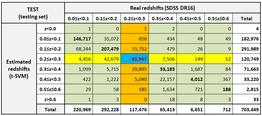
The performance variation of the t-SVM model with redshift can be roughly estimated by inspecting the values of the redshifts in sub-ranges of the latter. To this effect, a different class has been assigned to each redshift sub-range, both for the real and the predicted redshifts. Each redshift sub-range has a size of . The paradigm of a confusion matrix used in classification problems has then been applied. The matrix presents the total number of cases for each real class and each predicted one. Figure 11.61 illustrates the confusion matrix for the redshift ranges in the t-SVM, for the testing set.
The matrix constitutes the basis for the SVM performance metrics. For a given sub-range of real redshifts, , we consider as ”success” each case for which both the real and the estimated redshifts belong to this sub-range. The sum of these ”successes” gives the true-positive () value (blue cell in Figure 11.61) for this sub-range. If the real redshift belongs to , but the estimated one does not, we have a false estimation. The sum of all such cases (the column of orange cells in Figure 11.61) for this sub-range yields the false-negative value (). If the real redshift does not belong to but the estimated one does, we again have a false estimation. The sum of these cases yields the false-positive value (; the row of yellow cells in Figure 11.61) for the specific sub-range. Finally, the total sum of cases (all the green cells) where neither the real nor the estimated redshifts belong to defines the true-negative () value.
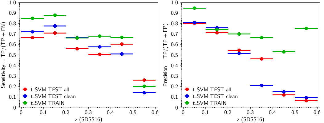
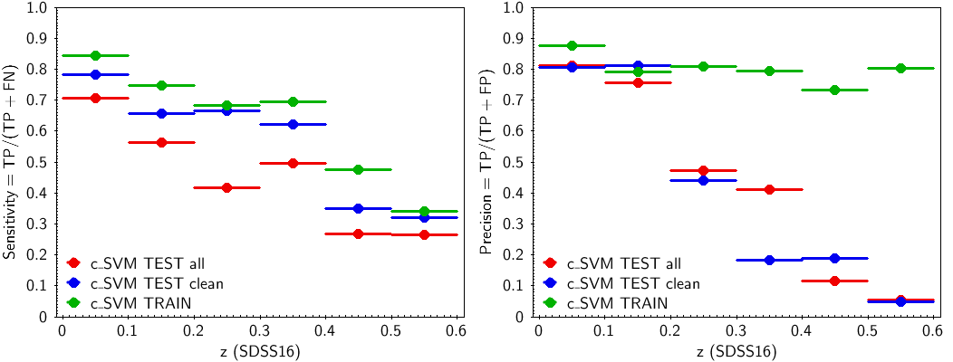
The values of , and are used to determine the t-SVM model performance for the six redshift sub-ranges: (i) the true positive rate, or sensitivity, or completeness, , and (ii) the positive predictive value, or precision, or purity, . Confusion matrices have also been created using in the performance tests the training data set and for the clean testing set, and the corresponding metrics parameters have been derived. Figure 11.62 shows the t-SVM sensitivity (left panel) and precision (right panel) values for the six redshift sub-ranges for the three data sets. Both precision and sensitivity are very good up to a redshift . The precision is marginal (0.5) for the two testing data sets for the redshift range 0.2-0.3 and fails at larger redshifts. The sensitivity is marginal in the range 0.3-0.5 and fails for the last sub-range. Generally, good performance can be expected up to redshifts .
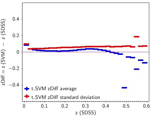
The redshifts estimated by the t-SVM module for the testing data set were split in sub-ranges in SDSS redshift with a step of 0.02.The mean and the standard deviation of the differences between the predicted and the real redshifts were determined for each sub-range. The two arrays give an estimation of the bias and the error of the redshift prediction, across the redshift range. Figure 11.63 shows the bias and error in dependence on the redshift subrange.
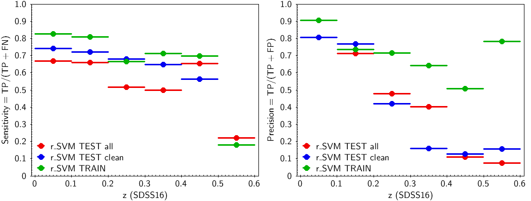
The same training and testing data sets have been used to prepare and validate the other two models used, the c-SVM and r-SVM. In these models, the target is not the redshift itself, but a code indicating the redshift sub-range of size in , within which the redshift lies. The c-SVM model is a classification SVM implementing C-SVC model type of LIBSVM. The training target is a numerically coded class for the redshift range: ”0” for , ”1” for , etc. up to ”5” for . The output is a class-probability vector. The element of the vector with the highest value above 0.5 defines the ”winner“ class, . If there is no element with probability larger than 0.5, is set to ”” which marks the source as unclassified. The second model used to predict the redshift range is a regression SVM, r-SVM, which implements the regression model -SVR of LIBSVM. It works like a pseudo-classifier. It is trained for discrete target values (0.0, 1.0, …, 5.0) where the value is defined by and converted to floating point. The integer part of the output is considered as the predicted redshift range numerical class, .
The performance of these models is shown in Figure 11.64. As different algorithms are implemented in c-SVM and r-SVM (classification and regression), they are used as an internal validation tool for the redshift value estimated by t-SVM (see Section 11.3.13).
Method
The UGC module consists of two sub-modules: UgcSelect and UgcSvmApply. UgcSelect checks each input source against three requirements for the source to be processed by UGC. The three requirements are:
-
•
the DSC Combmod probability for the source to be a galaxy is ,
-
•
the -band magnitude is in the range ,
-
•
the BP/RP sampled mean spectrum exists and the flux is defined for all the samples.
The source is rejected if any of the conditions fails, otherwise it is selected for processing.
UgcSvmApply processes each source that passed the selection. The sub-module applies the t-SVM model (see Section 11.3.13) to the sampled BP/RP spectrum of the source and estimates the redshift parameter, redshift_ugc and the index of the corresponding sub-range. Based on this result and using the t-SVM bias and error arrays, two parameters are defined by the sub-module for each estimated redshift, the redshift prediction limits given by:
| (11.39) |
Although the UGC module processes all selected sources, only the results for the ones that fulfill a predefined set of criteria are included in the archive. The criteria are grouped in two sets: “source applicability” and “redshift validity”.
The first group includes the conditions that need to be satisfied for the source to produce an usable redshift and are summarised in Table 11.35. Whenever one of these conditions is met, the corresponding flag is assigned value zero. The conditions are: The first condition requires that the number of transits used to produce the mean spectrum for both the blue and the red part is at least 10. The second condition sets specific lower and upper limits to the mean flux in BP and RP. The third condition revises the range adopted in the selection sub-module, by setting the bright limit to . This additional constraint aims to reject spectra of bright and possibly extended sources, for which it is likely that only part of the galaxy is recorded. The fourth condition imposes a lower limit to , to reduce as much as possible the number of high-redshift sources (). The fifth condition is related to location and concerns blended sources erroneously classified as galaxies in high density regions of the sky. The distribution of all the processed by UGC sources on the sky showed an unexpectedly high concentration of galaxies in three relatively small areas where distant extragalactic objects are not expected in large numbers: a region below the Galactic centre (CNT), and two areas centred on the Magellanic Clouds (LMC and SMC). Almost 9% of the processed sources originates in these three areas. It is noted that the sources in these three areas (CNT, LMC, SMC) occupy a specific region on the diagram, distinct from the locus of the remaining processed sources. This distinction has been used to define colour cuts which, in combination with the coordinates of the three areas, allowed us to clean the suspicious clumps of galaxies and effectively remove the sources in these three areas from the output table of UGC redshifts. This last condition is applied only if the DSC Combmod probability for the source to be a galaxy is less than .
| Flag | Condition |
| AND | |
| AND | |
| excluded are source falling in one of the CNT, LMC, SMC areas on the sky | |
| and in the specified colour-box (see details above) |
These conditions are combined in a cumulative flag, . When the value of this flag is zero (i.e. all individual flags are zero), the source is “acceptable”. The flag, Equation 11.40, is defined in such a way that it allows identification of the reason(s) for the rejection of a source.
| (11.40) |
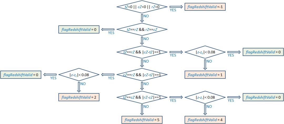
The second set of criteria concerns redshift validity. The criteria are based on the results from the different SVM algorithms applied in the t-SVM, c-SVM and r-SVM models (see Section 11.3.13). The first one yields a numerical value for the redshift, while the other two only provide a class corresponding to a redshift range of size 0.1. To make a direct comparison between the output of the three SVMs possible, we discretized the output of t-SVM by assigning it a code, , between “0” and “5”, defined by , where is the redshift value predicted by t-SVM. The code is then compared with the codes and derived from the application of the c-SVM and r-SVM models to the spectra.
This comparison yields the “redshift validity” flag, . If any of the three codes has a negative value (which means that no redshift class is assigned to the object by the specific SVM model) the redshift value (from t-SVM) is not validated, and the flag value is set to . If all three codes are equal, the redshift is validated and the value of the flag is set to 0. The redshift value is also validated (and the flag is set to 0) when two of the three codes have the same value, and the third one differs only by one (i.e. lies in a neighbouring range) and additionally the difference between the redshift value and the edge of the neighbouring range is less than 0.03 (or 0.08 from the centre of the neighbouring range), which is of the order of the standard deviation of the redshift values. The way this set of criteria is applied is described in the flow diagram of Figure 11.65.
Finally, the redshift value for a source is included in the output only if both the source acceptability and the redshift validity flags are equal to zero ( and ).
Outputs
The output is a Table (Section 20.5.1), which includes three fields, the redshift value and the redshift upper and lower prediction limits, as listed below.
redshift_ugc : The redshift of a source considered to be a galaxy by the Apsis module UGC. The redshift is estimated from the sampled mean BP/RP spectrum, by applying a regression model based on Support Vector Machines (SVM), which is a supervised machine learning algorithm (Section 11.3.13). The value of can be used as an estimate of the uncertainty in . For more details see Section 11.3.13.
The SVM redshift prediction limits (at -level) are based on the bias and the error , which are derived using the testing set (Section 11.3.13). The set is divided in a grid of sub-ranges of size 0.02 in real redshift. The prediction limits are then used as performance limits for a predicted redshift belonging to the corresponding sub-range (defined by ).
redshift_ugc_lower : The prediction lower limit is defined as
-
(see Equation 11.39).
redshift_ugc_upper : The prediction upper limit is defined as
-
(see Equation 11.39).
Scope
UGC processes sources having DSC combmod probability to be a galaxy larger than or equal to 0.25. The output is limited to galaxies with magnitudes in the range and is filtered
Results
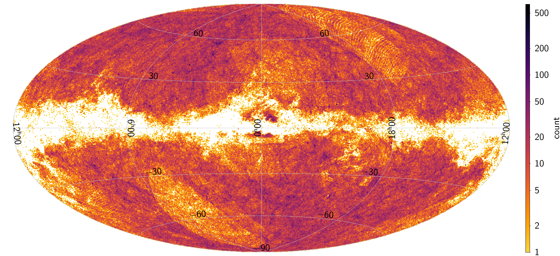
The table galaxy_candidates includes 1,367,153 sources with redshifts estimated by UGC. Excluding the Galactic plane areas, the sources are almost randomly distributed on the sky (see Figure 11.66), although there are two areas (lower-left and upper-right) of relatively lower density of UGC sources displaying characteristic residual patterns. These are regions which have been observed fewer times and thus many of the sources in them do not appear in the UGC output because of the acceptability conditions applied (see Table 11.35).
The redshift distribution has a maximum at around 0.1, with very few sources with redshifts above 0.25. The lowest and the highest redshifts in the table are and , respectively. There are 33 sources with negative redshifts, although most of these values are very close to zero. Table 11.36 shows the number of sources in redshift bins of 0.05. The distribution of redshifts is illustrated on the left panel of Figure 11.67. The dependence of the predicted redshift on G magnitude is shown on the right panel of Figure 11.67. Generally, higher redshift sources are fainter, as expected.
| Sources | 24 960 | 344 928 | 461 407 | 295 755 | 141 405 | 42 950 |
| % | 1.83 | 25.23 | 33.75 | 21.63 | 10.34 | 3.14 |
| Sources | 31 982 | 15 173 | 6 015 | 2 037 | 481 | 60 |
| % | 2.34 | 1.11 | 0.44 | 0.15 | 0.04 | 0.00 |
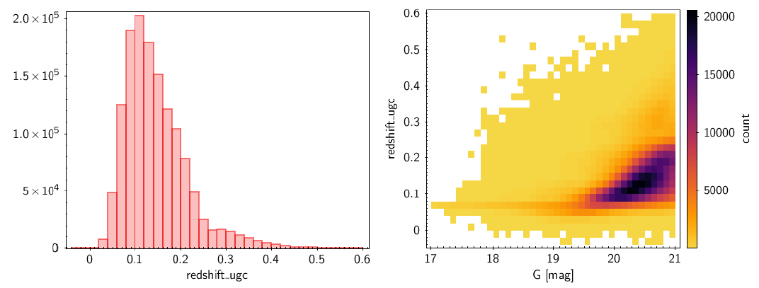
Diagram / counts and weighted by redshiftUgc Figure 11.68
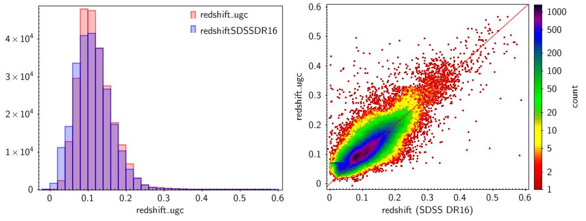
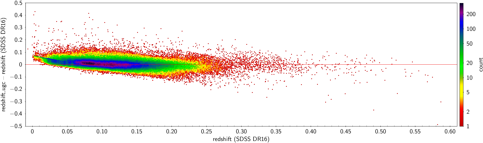
There are 248 356 sources in the galaxy_candidates table in common with the SDSS DR16 extragalactic sources (see Section 11.3.13) . The difference between the estimated by UGC and the reference (SDSS) redshifts has a mean and standard deviation of and , respectively. If the 67 sources with reference redshifts greater than 0.6 are excluded, the standard deviation reduces to . Figure 11.69 (left panel) compares the two redshift distributions, the reference SDSS redshifts (in blue) and the UGC estimated redshifts (in red). Generally, there is good agreement, although there is an excess of UGC redshifts around 0.1 probably due to an overestimation of lower redshifts. On the right panel,the redshifts estimated by UGC are plotted against SDSS DR16 redshifts. In this diagram, there is a clear excess of estimated redshift values around 0.07 (a small horizontal branch) for sources with reference redshifts below this value.
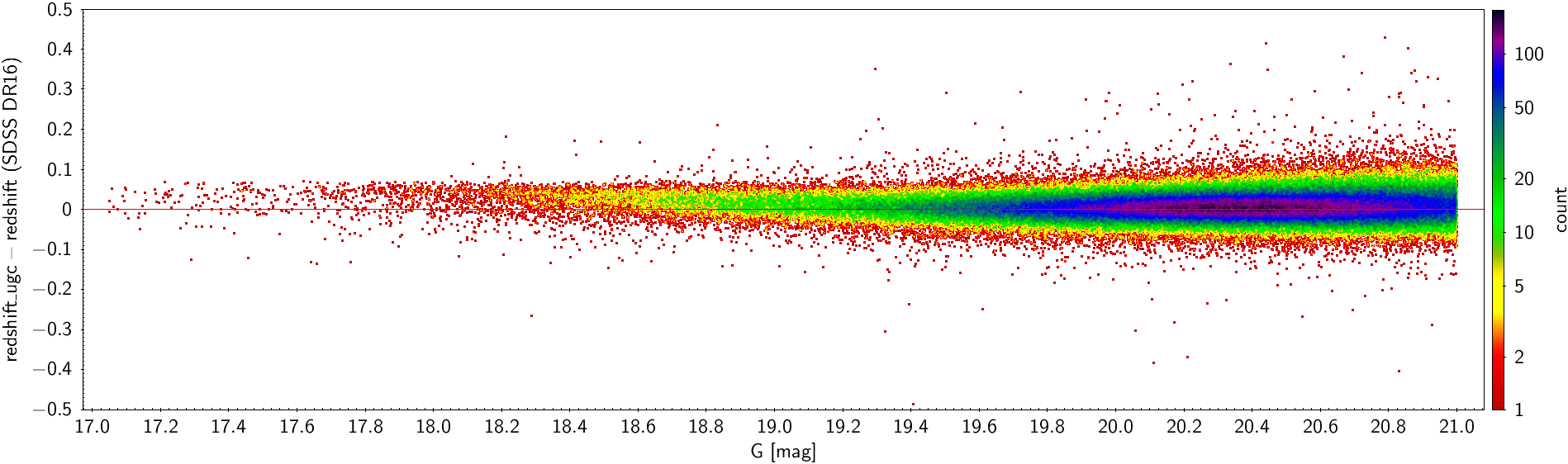
Because of the previously mentioned lack of balance in the redshift distribution of the SVM training set, the performance of the UGC redshift estimator is not constant over the entire redshift range, as is evident in Figure 11.70. The differences between predicted and reference redshifts tend to be positive for small redshifts and negative for larger ones. As expected, the performance of the UGC redshift estimator is worse for fainter sources as shown by the increase in the difference between the predicted and the reference redshift for larger G magnitudes (Figure 11.71).
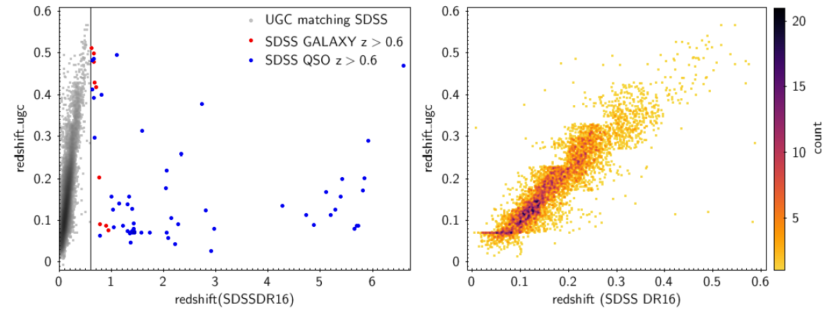
UGC selects sources which have a value larger than 0.25 for the DSC combined probability for a source to be a galaxy. As a result, the final UGC galaxy catalogue is expected to include some misclassified quasars. Indeed, 5 000 sources, or of the testing set (i.e. of the sources in common in the UGC catalog and the SDSS DR16 extragalactic object catalog) have an SDSS “QSO” classification. About one percent of these QSOs have redshifts higher than the UGC limit ().
Figure 11.72 (left panel) shows a comparison between UGC and SDSS redshifts for high redshift QSOs (in blue) and high redshift galaxies (in red).
As expected, the t-SVM model prediction is unrealistic, as it is necessarily limited to . However, the agreement between UGC and SDSS redshifts for QSOs with redshifts below 0.6 is good, despite the fact that the SVM was not trained for quasars (right panel of Figure 11.72).
Use
A few important remarks on the content of the UGC redshifts in the integrated galaxy table.
-
•
The definition of a source as a galaxy in UGC is based on the DSC Combmod probability for the source to be a galaxy, namely .
-
•
About of the sources are expected to be misclassified quasars. Although the module has not been prepared (trained) for such objects, the redshift prediction performance is only slightly worse than for galaxies, for .
-
•
For QSO contaminants with large redshifts (), the estimated redshift is completely wrong. It is expected that nearly one percent of the QSOs inadvertently included in the UGC catalog are high-redshift sources.
-
•
There are also high-redshift galaxies in the UGC output, but their number is negligible.
-
•
Estimated redshifts larger than 0.4 are questionable. This is caused by the small number of galaxy spectra beyond that are available for the SVM training.
-
•
Redshifts close to zero, are also unreliable because of the large prediction error of the SVM model in this regime.
-
•
A suspicious large peak of sources is shown in the redshift bin . As many as sources are found there. Almost 4 000 have a redshift value . It is estimated that most of the galaxies in the peak have real redshifts below 0.04. A large part of the contaminating sources () can be discarded by applying magnitude cuts in this bin: , and .