11.3.5 Multiple Star Classifier (MSC)
Author(s): Jan Rybizki
Goal
The multiple star classifier (MSC) infers stellar parameters for all sources brighter than mag from low-resolution BP/RP spectra and parallaxes under the assumption that the source is an unresolved coeval binary system with a flux ratio below 5 (flux ratio - primary BP/RP total flux divided by secondary BP/RP total flux, the primary being defined as the brighter component in BP/RP flux). In particular it provides and estimates for each of the two components, as well as , and distance for the pair (i.e. are assumed the same for both components). These parameters are directly sampled in an MCMC, but we also provide the derived quantity as well as MCMC quality parameters. The likelihood is based on a comparison between data and model using a BP/RP spectra forward model grid which has been generated empirically using APOGEE stellar parameters (Holtzman et al. 2015) (in contrast to GSP-Phot, where the forward model grid is based on simulations see Section 11.3.3).
Inputs
As Gaia data inputs MSC requires both BP and RP spectra and uses the normalised flux together with the associated uncertainties which we increase by a factor of 2, in order to increase the influence of the parallax measurement. Furthermore, MSC makes use of the total BP/RP spectra flux and the parallax taking the zero-point parallax correction into account, which is implemented via SMSgen, see Section 11.3.1.
External inputs needed for the distance prior and extinction parameter upper limits per HEALPix are taken from GeDR3mock ADQL queries (Rybizki et al. 2020). Furthermore a flux ratio prior and HRD prior are based on the wide binary sample (El-Badry and Rix 2018). The stellar parameters for the individual components of these wide binaries have been inferred using PARSEC isochrones (Marigo et al. 2017) and a 3D extinction map both explained in Rybizki et al. (2020). The parameter inference framework, based on the assumption of the wide binaries being coeval, is sketched in this notebook (this is in principle a minimal python version of MSC only using photometry instead of BP/RP spectra). We sum the individual components’ BP/RP spectra of the wide binary sample in order to train a machine learning algorithm that helps to initialise the MCMC chain.
Method
The main algorithm in MSC is double Aeneas (in analogy to the single star GSP-Phot algorithm called ’Aeneas’), which uses a BP/RP forward model together with an ensemble MCMC algorithm (Foreman-Mackey et al. 2013) to sample the posterior. Its optimisation parameters are effective temperature for both components & , surface gravity for both components & , metallicity , extinction and distance. During the computation of a single posterior point double Aeneas first takes a precomputed BP/RP spectra grid and uses 4D linear interpolation over , , and to obtain a model BP/RP spectrum for the first component. Then it does the same for , , and to get a model spectrum for the second component. From these two model BP/RP spectra the flux ratio is calculated and the spectra are summed and scaled by the last free parameter, i.e the distance. Then a of the normalised BP/RP spectra, the total BP/RP flux and the parallax (i.e. 1/distance) is computed. The overall is thus calculated from 242 data points (240 BP/RP pixels, 1 total BP/RP flux and 1 parallax measurement) and their associated uncertainties (we increase the BP/RP spectra uncertainties by a factor of 2). The 4D linear interpolation over , , and not only produces a model BP/RP spectrum but also a corresponding extinction , which we also report. This ensures that all extinctions are consistent with the underlying model SED and no transformation relations are needed.
In the posterior probability, which is sampled by the double Aeneas MCMC, the following priors are in place:
- •
-
•
A Gaussian prior on with mean = 0 and standard deviation of 0.2 dex.
-
•
Extinction prior of exp( mag) with the further addition of a maximum , coming as well from GeDR3mock.
-
•
A BP/RP spectra flux ratio prior that peaks towards equal flux binaries in the range of 1flux ratio5, coming from the flux ratio distribution of the wide binary sample (El-Badry and Rix 2018).
-
•
a – plane prior (HRD prior) for both components, derived from the wide binaries primary components parameters.
The initial guess for the double Aeneas MCMC is obtained from extremely randomised trees (ExtraTrees) (Geurts et al. 2006), which is a machine-learning algorithm, that we trained on the wide binary (superimposed BP/RP spectra) sample, see Section 11.3.5.
Instead of simulated libraries as used by GSP-Phot, MSC uses an empirical BP/RP spectra forward model grid. We train an ExtraTree model on the BP/RP spectra of 80k APOGEE sources (Holtzman et al. 2015) that have both ASPCAP (Jönsson et al. 2020) and StarHorse (Queiroz et al. 2020) parameters. This omits problems in the calibration of the BP/RP spectra instrument model (too few calibrators in the blue end are used) but relies on the APOGEE parameters and by construction is noisier than a simulated grid. With this ExtraTree model we predict the gridpoints of our 4D BP/RP forward model grid, which is then used within double Aeneas as the BP/RP forward model via linear interpolation. The BP/RP grid points are:
-
•
range: 2.0 - 5.2 dex in steps of 0.1dex.
-
•
range: 3,000 - 8,000K in steps of 100 to 200K.
-
•
grid points are: -1. -0.7 -0.5 -0.3 -0.2 -0.1 0. 0.1 0.2 0.3 0.5 dex.
-
•
grid points are: 0. 0.1 0.2 0.3 0.4 0.5 0.6 0.7 0.8 0.9 1. 1.2 1.4 1.6 1.8 2. 2.4 2.8 3.2 3.6 4. 4.4 5. mag.
This also shows the parameter ranges of the double Aeneas inference. For the distances we require: 1 log10(distance/pc) 4 (i.e. 10 pc to 10 kpc). is also sampled in log space.
Outputs
The MSC results are available in the astrophysical_parameters. There are also 100 random MCMC samples for each source available in a separate table mcmc_samples_msc via DataLink. Whether a source has MSC results is indicated in the gaia_source field has_mcmc_msc. If a result exists then all fields of MSC are filled. We provide upper and lower 1 confidence intervals, i.e. 16th and 84th percentiles, together with the median value for all sampled parameters, i.e. effective temperature for both components & (in K), surface gravity for both components & (in dex), metallicity (in dex), extinction (in mag) and distance (in pc). In the MCMC chain we additionally provide the log posterior (log = natural logarithm) and the log likelihood for each sample such that the log prior value can be reconstructed. The uncertainties have been increased by a factor of 10 (e.g. upper-median times 10) in the reported confidence intervals (respecting the respective parameter limits), but we have not altered the values in the MCMC chains. The scaling factor of 10 for the uncertainties was empirically determined when trying to make the mutual uncertainties with the GALAH data set compatible. For the parameter , which has not been optimised for in the MCMC but is a derived quantity, we also report median values and upper and lower confidence intervals.
Additionally we provide MCMC quality indicators: mcmcaccept_msc reports the mean acceptance fraction over all 100 walkers (we used at least 175 burn-in steps and 145 fitting steps, thinning to 100 samples was applied before computing the summary statistics). The logposterior_msc parameter gives the mean log posterior over the MCMC samples. The mcmcdrift_msc parameter is a proxy for the convergence of the MCMC chain and reports the mean parameter drift (over all seven parameters) of the stabilized MCMC chain normalized by the 10 times inflated parameter uncertainty (as given by the final 100 MCMC sample’s standard deviation). Finally the flags_msc field, which is a string (all other fields are floats) indicates very bad MSC solutions, by flagging any source with ’1’ that has either logposterior_msc or mcmcdrift_msc . All other sources are flagged with ’0’.
Scope
MSC has processed all sources with that have a parallax and a BP/RP spectrum. No filtering has been imposed, but the flags_msc field marks around 13 % of the 350M sources as having poorly converged MCMC chains. We do not provide any information whether a respective source actually is an unresolved binary; we just provide the best parameter fits assuming it is. So the user will have to use external data to collect a sample of applicable MSC binaries for which they can then extract the relevant parameters. It might also be possible to use colour-absolute magnitude diagram (CAMD) cuts to select likely equal mass binaries (i.e. binary main sequence) or combine other Gaia parameters to select a sample of binaries in specific parameter ranges. Generalising this problem to all binaries has not yet been successfully implemented within Apsis.
Results
As an independent validation set we use 10k GALAH (Martell et al. 2017) binaries (Traven et al. 2020a) that have a flux ratio of less than 5 and are within the double Aeneas’ BP/RP forward model grid ranges. The comparison is depicted in Figure 11.27, where the colour code shows the mean log posterior, i.e. no density information is given. From top to bottom the following parameters are compared. , & , , , , distance and .: For all but extinction we see that the goodness of fit, i.e. the logposterior_msc parameter is best towards the 1 to 1 line. This shows that the empirical grid used as a forward model during the MSC inference does a solid job.
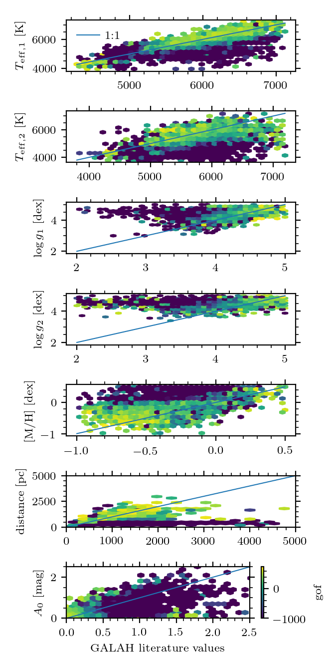
If we impose cuts on the logposterior_msc quality indicator the quality of the inferred parameters improves significantly as can be seen from the root-mean-square error (RMSE) values in Table 11.25.
| logposterior_msc lower limit percentiles | 0 | 5 | 16 | 50 | 84 | 95 |
| limiting logposterior_msc values | -201 147 | -4 437 | -596 | 488 | 689 | 752 |
| sourcecount | 11 263 | 10 699 | 9 461 | 5 637 | 1 814 | 567 |
| parameters | sample RMSE | |||||
| 387 | 348 | 273 | 192 | 144 | 135 | |
| 632 | 592 | 536 | 417 | 310 | 258 | |
| 0.40 | 0.35 | 0.33 | 0.29 | 0.25 | 0.24 | |
| 0.58 | 0.54 | 0.50 | 0.45 | 0.38 | 0.36 | |
| 0.30 | 0.29 | 0.27 | 0.24 | 0.22 | 0.21 | |
| distance | 617 | 553 | 277 | 152 | 47 | 25 |
| 0.27 | 0.24 | 0.21 | 0.19 | 0.15 | 0.13 | |
| sample bias | ||||||
| -139 | -118 | -72 | -6 | 21 | 10 | |
| -418 | -392 | -350 | -245 | -144 | -60 | |
| 0.24 | 0.22 | 0.20 | 0.17 | 0.13 | 0.12 | |
| 0.35 | 0.33 | 0.30 | 0.24 | 0.17 | 0.15 | |
| 0.21 | 0.20 | 0.19 | 0.19 | 0.19 | 0.18 | |
| distance | -184 | -148 | -95 | -49 | -16 | -9 |
| -0.01 | 0.00 | 0.01 | 0.02 | 0.01 | 0.01 | |
Similarly the bias decreases with increasing logposterior_msc cut-off. A remarkable difference between GALAH and MSC parameter estimates is the persistently higher values for , and , offsets that do not improve much with higher logposterior_msc. The physical/model mechanism behind this is the balance between higher metallicity values (that increase the luminosity) and the higher values (that decrease luminosity). It could be that the MSC prior (Gaussian with mean at 0 dex) on metallicity pushes our inference into that direction. On the other hand the GALAH binaries distribution is relatively metal-poor for a disk sample. It could be that binary parameter inference is particularly sensitive to model assumptions, which can easily result in systematic offsets. Another indication for this model dependence are low correlations between inferred parameters for 26 sources in common between the GALAH sample and the APOGEE binary sample (El-Badry et al. 2018).
So far we have only validated the median values of the MCMC chain. When looking at the difference between MSC results with GALAH normalised by their reported uncertainties we see that they are strongly incompatible, which is very likely due to a combination of MCMC convergence issues and underestimated model uncertainties. We correct for that empirically by inflating the MSC uncertainties by a factor of 10 (respecting the respective parameter ranges) which brings the residual distribution closer to the expected one, at least for sources with well-behaved logposterior_msc values. Still the distribution of the normalised differences between MSC and GALAH is stronger peaked than a normal distribution and has wider tails.
Use
Since MSC assumes all sources are binaries, and DSC (Section 11.3.2) does not provide a useful identification of unresolved binary stars, all use-cases should start with a sample of already known binaries or at least good binary candidates. As can be deduced from Figure 11.27, the MSC inference is unreliable when one component is a giant, as well as for sources with high extinction. The uncertainties have been inflated in order to be compatible with the GALAH comparison, i.e. give a realistic idea about the true uncertainties. The extinction values are not well determined for high extinctions ( ). The other parameters are reasonably well determined especially for sources with large logposterior_msc. The MCMC samples list all model parameters, as well as the likelihood and posterior, from which the prior could be computed to within a normalization constant. Thus it would be possible for the user to compute parameter correlations and also compute summaries of the posterior. Results of other non-single star modules of Gaia DR3 can of course be combined/augmented with MSC results. Our inferred parameters can also be used as an initial guess for subsequent inferences. One might even be able to find binaries (for subsets of the binary parameter space) by comparing goodness-of-fit measures from GSP-Phot and MSC (possibly in combination with other Gaia data products, e.g. ruwe).