11.2.3 Use of BP and RP spectra in CU8

A set of libraries of synthetic and semi-empirical spectra are used to train several Apsis modules, and include stellar, galaxy and QSO spectra. The spectra cover the 300–1100 nm wavelength range, with 8001 flux points sampled every 0.1 nm.

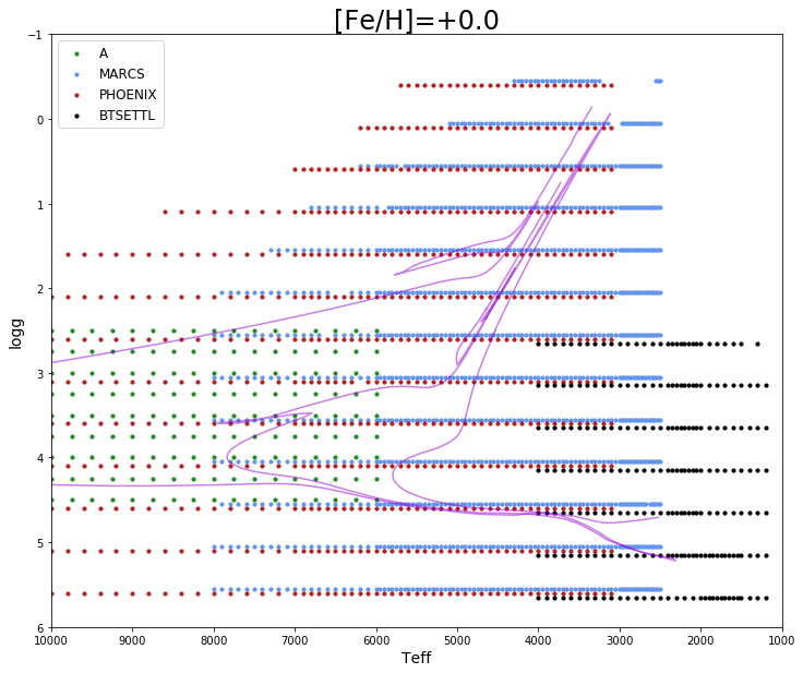
The synthetic stellar libraries cover the HR diagram as much as possible, at discrete steps. The different model families are computed using different assumptions, from different physical ingredients (chemical composition) to the treatment of specific processes (see Bailer-Jones et al. (2013)). Their coverage in significant parameters ($T_{\mathrm{eff}}$, $\log g$, metallicity) is shown in Table 11.13. Furthermore, we emphasise that all synthetic stellar libraries have their spectra normalised such that their total integrated flux (including wavelengths outside 300-1100nm) satisfies the Stefan-Boltzmann law, i.e. the flux levels are such that the total integrated flux scales with ${\sigma }_B{T}_{\mathrm{eff}}^4$. In the following, we summarize some basic information on the libraries used by Apsis modules in DR3.

Hereafter we summarize the basic model family characteristics:

• •

  MARCS These models are described in detail by Gustafsson et al. (2008). For $\log g\le$ 3.5, spherical models are computed with 1 ${ℳ}_{\odot }$ and microturbulence parameter=2  $\mathrm{km}{\mathrm{s}}^{-1}$, while for dwarf stars plane-parallel models are computed, with microturbulence parameter=1  $\mathrm{km}{\mathrm{s}}^{-1}$. Solar abundances are from Grevesse et al. (2007). The library is provided at very fine step in $T_{\mathrm{eff}}$, especially at low temperatures where non-linear effects make interpolation more prone to errors.

• •

  PHOENIX details are given in Brott and Hauschildt (2005)

• •

  LL models are used to simulate B-F stars, see Shulyak et al. (2004), and implement direct computation of line opacity. Solar abundances are from Asplund et al. (2009)

• •

  OB spectra are computed from the model atmosphere grids available on the TLUSTY website (Lanz and Hubeny 2003, 2007). A microturbulence of 2 $\mathrm{km}{\mathrm{s}}^{-1}$ was considered for models cooler than 30000 K, and of 10 $\mathrm{km}{\mathrm{s}}^{-1}$ for the hotter ones.

Many other spectral libraries (synthetic or semi-empirical) have been computed and provided to CU8, but either used only internally for algorithm preparation/validation or not yet implemented in the processing. Among those: Be (B stars with emissions) and WR stars, Physical Binaries, WD stars.

Extragalactic sources are simulated using the following libraries: Galaxies EMP, Galaxies SE, Galaxies E,I,Q,S, Outliers, RadioFirst, SDSS QSO. All Galaxy libraries are used by UGC (Section 11.3.13). The SDSS QSO is used by QSOC (Section 11.3.14). The Outliers and RadioFirst librarires are used by the OA (Section 11.3.12).

Bolometric corrections (BC) are calculated for the MARCS and OB libraries. BCs are needed in FLAME processing, see Section 11.3.6. They are computed from the spectra using the Gaia EDR3 passbands, either via integration over all wavelengths (for standard MARCS and OB) or by using the Stefan-Boltzmann law for the LL models. A bolometric correction tool is available on the Gaia DR3 software and tools webpages.

Based on the $T_{\mathrm{eff}}$, $\log g$ and $[\mathrm{M}/\mathrm{H}]$ of the synthetic spectrum, we assigned the fundamental parameters (luminosity, mass, radius…) using Padova evolutionary models, on a best-match approach. This means that we generated a very large population of stars, spanning all available ages and metallicities (in the models), and looking for the closest match in this population. A flag indicates if this match is satisfactory, based on a threshold on the geometrical distance between the point and the best-match. This threshold is variable according to the spectral type of the star.

Observed spectra are attenuated (i.e. dimmed and reddened) by the amount of interstellar dust present between the observer and the source, so if $F(\lambda )$ is the source spectral energy distribution, $A(\lambda )$ is the extinction curve, then the attenuated, observed flux $f(\lambda )$ is:

In this sense, extinction can be considered an astrophysical parameter of a given source, and can be inferred using the spectra. To properly train the algorithms, simulations must be provided at different levels of extinction.

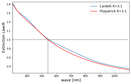
We adopted the wavelength dependent extinction law of Fitzpatrick (1999), which is parametrized by $A_V$, the extinction in the $V$ band, and $R\equiv A_V/E(B-V)$. Specifically, they provide a numerical recipe for generating values of $A^{\prime }(\lambda )=[A(\lambda )/E(B-V)]$, the extinction law normalized to a colour excess of E(B-V)=0.5 for a 30.000 K star, letting the user specify the parameters $A_V$ and $R$ to derive a specific extinction curve $A(\lambda )=A_V{A}^{\prime }(\lambda )/R$. (We note that in this context $A_V$ and $R$ are to be understood as extinction parameters.) In our application of the Fitzpatrick extinction law we fix R=3.1, and note that $[A^{\prime }(\lambda )/3.1]$ is equal to 1 at the specific wavelength 541.4 nm (see Figure 11.3) , so that we can define the extinction parameter $A_0$ as the monochromatic extinction at 541.4 nm and

The extinction curve at R=3.1 used in CU8 simulations is available together with the parameter files on the Gaia DR3 auxiliary data webpage.

For each spectral energy distribution, the extinction in a given band is computed by integrating the spectra $F$ and $f$ (i.e., with and without applied extinction) over the chosen passband, to obtain the integrated fluxes. Using the Gaia $G$ band as an example, we derive:

and

where $T_G$ denotes the transmission of the $G$ passband. We then take the ratio of $F_G$ and $f_G$ and compute the magnitudes. This is equivalent to:

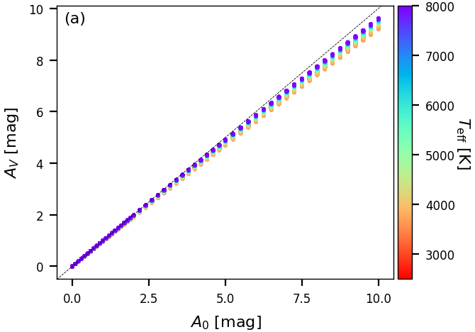
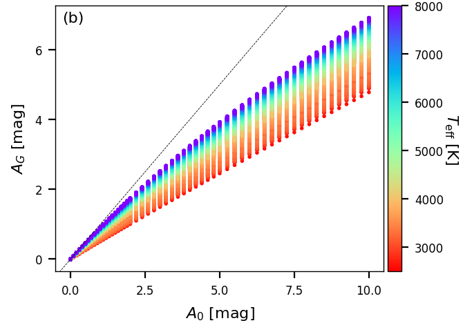
The same procedure is used to compute extinction coefficients $A_{\mathrm{BP}}$ and $A_{\mathrm{RP}}$ for the Gaia $G_{\mathrm{BP}}$ and $G_{\mathrm{RP}}$ passbands. For internal use and to check consistency, we also compute extinction coefficients in the Johnson B, V, I bands (Bessell 1990). These values are not published in Gaia DR3. We explicitly note the intrinsic difference between the extinction parameter $A_0$ and the extinction in the Johnson $V$ band $A_{\mathrm{V}}$, while these two notations are often confused in the literature. In particular, the actual extinction in a given band is coupled with the spectrum of the emitting source: i.e. a given $A_0$ corresponds to different values of $A_{\mathrm{V}}$ for stars having a different spectral type, as shown in Figure 11.4a. As is evident from Figure 11.4b, the same effect also applies to $A_{\mathrm{G}}$, but since the Gaia $G$ band is significantly broader than the Johnson V band, the effect is even more pronounced in $A_{\mathrm{G}}$ than in $A_{\mathrm{V}}$.

CU5 (P. Montegriffo) provided a simulator that implements the instrument model and the extinction law as derived through the BP/RP spectra external calibration process in CU5, see Chapter 5 for more details. The tool takes a model spectrum as input and gives an instrument spectrum as output, in the same format as the BP/RP spectra from CU5. The BP/RP spectrum simulator uses the Gaia EDR3 photometric passbands to compute the Gaia photometry from the spectra.