11.3.2 Discrete Source Classifier (DSC)
Author(s): Coryn A.L. Bailer-Jones
More information on DSC, in particular the results, can be found in Bailer-Jones (2021), Gaia Collaboration et al. (2023b), and Delchambre et al. (2023).
Goal
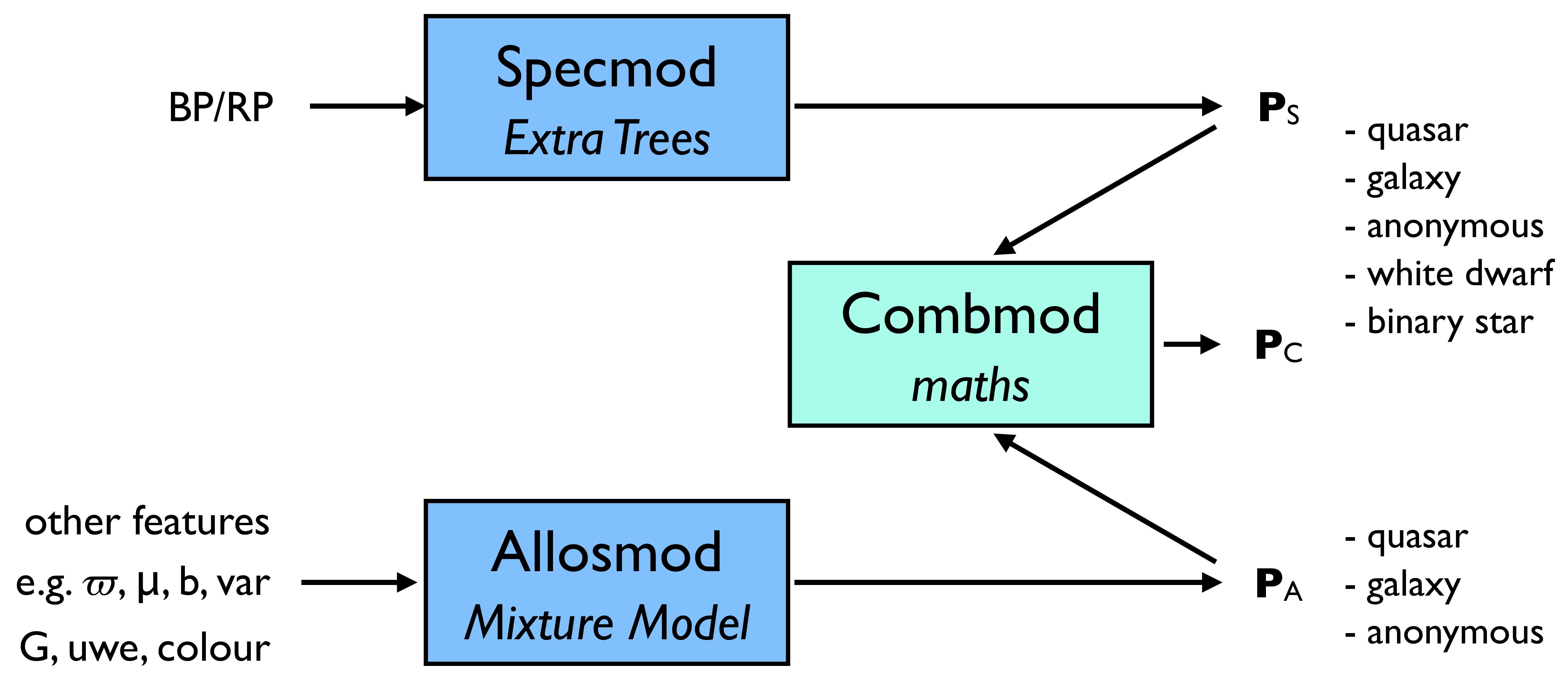
DSC classifies Gaia sources probabilistically into five classes: quasar, galaxy, star, white dwarf, physical binary star. These classes are defined by the training data (see Section 11.3.2), which are Gaia data with labels provided by external catalogues. Hence DSC is empirical (sometimes called ”data driven”). DSC comprises three classifiers (see Figure 11.6): Specmod uses BP/RP spectra to classify into all five classes; Allosmod uses various other features to classify into just the first three classes; Combmod takes the output class probabilities of the other two classifiers and combines them to give probabilities in all five classes.
Training data
DSC is trained empirically, meaning it is trained on a labelled subset of the actual Gaia data it will be applied to (except for binary stars, as will be explained). The classes were defined by selecting sources of each class from an external database and crossmatching them to sources in Gaia DR3. A subset of these data were then used to train, another to test. The sources used to define each of the five classes are as follows. For more details see Bailer-Jones (2021).
- Quasar.
-
SDSS-DR14 quasar catalogue (Pâris et al. 2018). This is the same catalogue as used in Bailer-Jones et al. (2019) and is nominally the same subset, obtained with
SDSS_NAME!="00000-00000" AND ZWARNING=0
which gave 446 492 rows (not necessarily unique sources). We positionally crossmatched this to Gaia using a 1 radius. All sources were retained that had both phot_bp_n_obs and phot_rp_n_obs equal to or greater than 5. This gave 349 876 sources. - Galaxy.
-
SDSS-DR15 spectroscopic catalogue (Aguado et al. 2019). This is the same catalogue as used in Bailer-Jones et al. (2019) and is nominally the same subset, obtained with
class='GALAXY' AND subClass!='AGN' AND subClass!='AGN BROADLINE' ANDzWarning=0
which gave 2 312 057 rows. We then performed a crossmatch to Gaia and took the subset in the same way as done for the quasars. This gave 715 739 sources. - Star (anonymous).
-
Objects drawn at random from Gaia DR3 that are not in the quasar or galaxy training sets. Strictly speaking this is therefore an ”anonymous” class. But as the vast majority of sources in Gaia are stars, and the majority of those will appear in (spectro)photometry and astrometry as single stars, we call this class ”stars”.
- White dwarf.
-
All white dwarfs from the Montreal White Dwarf Database that have coordinates and that are not known to be binaries (using the flag provided in that table; downloaded 2020-04-22). This was crossmatched to Gaia, and sources selected, in the same way as for the quasars. This gave 48 819 sources.
- Physical binary star.
-
From a set of spatially resolved binaries with differences less than 3.0 mag, the separate BP/RP spectrum of each pair was combined into a composite single spectrum to represent the spectrum of an unresolved binary. In principle any two BP/RP spectra could be used for this, but components of a real binary were taken to ensure they have real – if restricted – mass and luminosity ratios, and had the same interstellar extinction. The input catalogue for this was a set of 200 000 binaries identified in Gaia DR2 by El-Badry and Rix (2018). For training DSC, the sample was further limited to (a) those synthesized binaries that have flux ratios between 1.5 and 5, and (b) those for which both components have colours within the range 0–1.3 mag (roughly corresponding to a range of 3000–10 000 K). This gave 89 129 synthesized binaries for training/testing. Note that this is the only class which does not use Gaia data directly.
The following filters were then applied to the data on all classes:
-
•
Remove duplicate sources.
-
•
Remove apparent stellar contaminants from the galaxies, by removing all sources from the galaxies that have (see Bailer-Jones et al. 2019)
. -
•
Remove intrinsically bright sources from the white dwarfs by removing from this class all sources with
where is the parallax in mas.
This gave a total of about 700 000 sources across all classes. A subset was selected for the training, and a similar-sized disjoint subset was used for testing.
Only those quasars, galaxies, and star sources that had a complete set of Allosmod features (Section 11.3.2) and complete BP/RP spectra, i.e. no missing data, were used for training and testing both Specmod and Allosmod. Thus the same set of quasars, galaxies, and stars were selected for training/testing Specmod and Allosmod. The only exception to this is that sources with mag were not used to train Allosmod. This is because Allosmod classifies such bright sources as a star, i.e. assigns this class a probability of 1.0.
It is important to appreciate that the classes are defined by these training data. Thus “galaxy” is not any galaxy, but one with Gaia data that are consistent with the galaxies in our training set. This is particularly relevant for the “physical binary” class, as this represents a very small subset of all types of physical binary one could think of and which Gaia no doubt observes.
Inputs
The input to Specmod is the BP/RP spectra as sampled by SMSgen with 60 samples in each of BP and RP. The first and last five samples of each of BP and RP are excluded, leaving 100 input elements.
The inputs to Allosmod are eight features formed from fields in Gaia source table (the field names are links to the data model):
-
•
sine of the Galactic latitude,
-
•
parallax, parallax
-
•
total proper motion, pm
-
•
unit weight error (uwe),
-
•
band magnitude, phot_g_mean_mag
-
•
colour , bp_g
-
•
colour , g_rp
-
•
The relative variability in the band (relvarg),
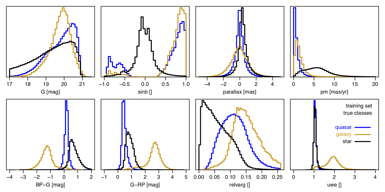
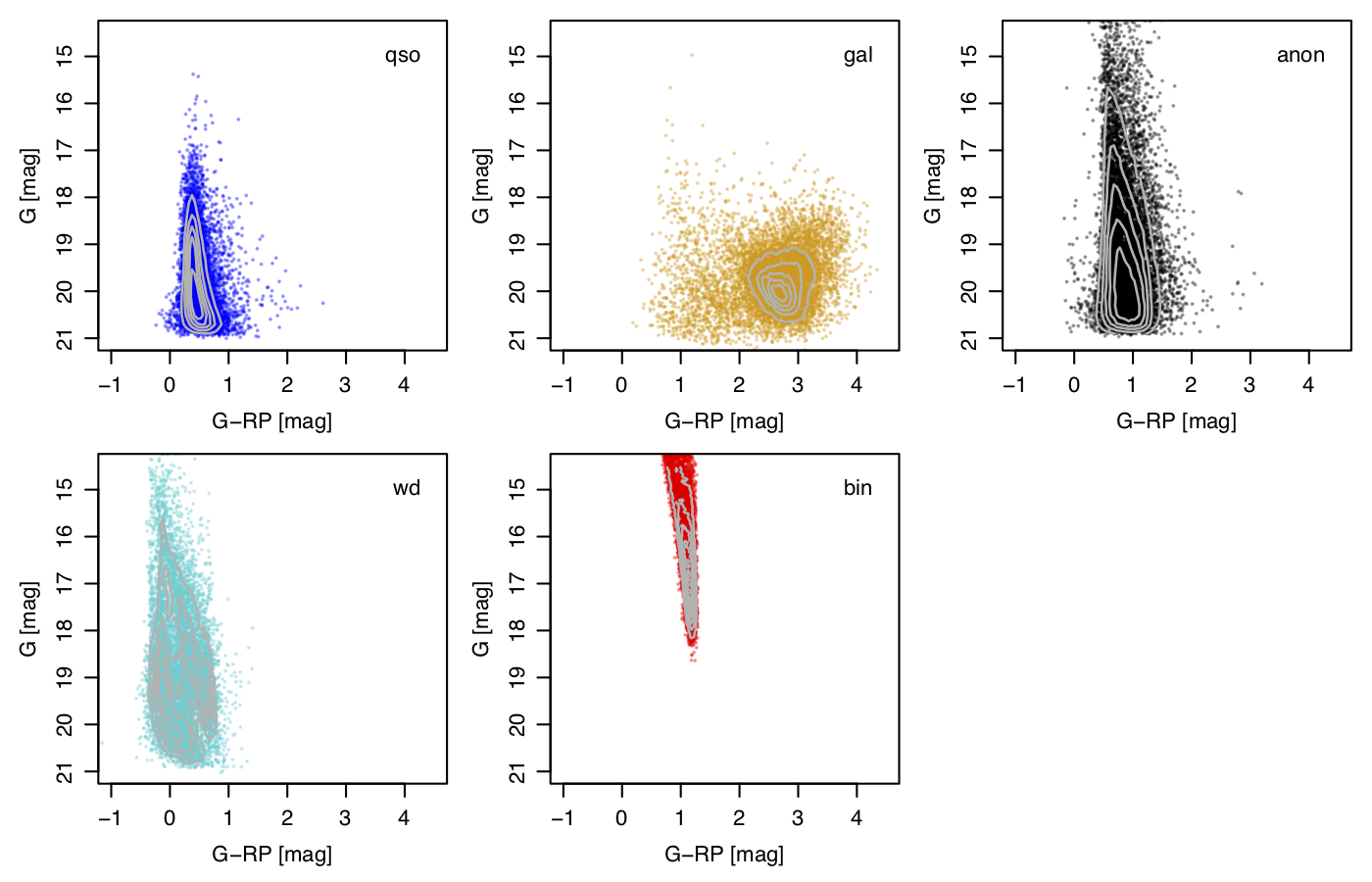
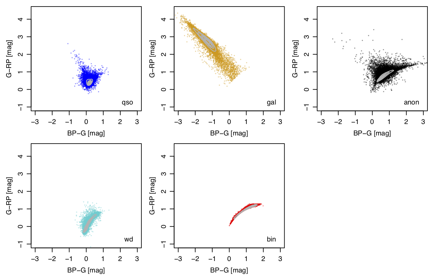
Figure 11.7 shows the distribution of these eight Allosmod features for the training data for each of the three classes used in Allosmod. Each feature helps distinguish between the classes in different ways. The use of the colours and magnitudes is an obvious choice: these are also illustrated in the colour–magnitude and colour–colour diagrams in Figure 11.8 and Figure 11.9 The ratio of the true number of extragalactic to galactic objects visible to Gaia varies with Galactic latitude. The actual latitudes of the quasars and galaxies in our train/test sample are an artefact of the SDSS selection function. We therefore replace their values with values drawn from a uniform distribution for the sake of model training, to avoid that our model learns the SDSS footprint. When applying the trained DSC model to the unlabelled Gaia data to make the catalogue, the measured values of the sources are of course used. The large values of the parallax, proper motion, relvarg, and uwe for galaxies in Figure 11.7 occur because many galaxies are spatially resolved by Gaia. This leads to a different centroid being determined by the on-board detection algorithm each time the galaxy is scanned. These large shifts are sometimes fitted as spuriously large parallaxes and proper motions by AGIS. This may be indicated by a large value of uwe, which is why we also use this as an input. This variable centroiding from epoch to epoch can also induce a spurious variability in the measure photometric flux, thereby producing large values of relvarg. By including all these features as inputs, DSC-Allosmod can take advantage of these ”failures” to help identify galaxies, and to a lesser extent quasars too.
For each source, Combmod takes the probabilities computed by Specmod and Allosmod, and computes new probabilities, as explained in Section 11.3.2.
Outputs
For each source, DSC produces three normalized posterior probability vectors, one for each of the classifiers Specmod (5 classes), Allosmod (3 classes), and Combmod (5 classes). DSC also produces two class labels derived from these probabilities (explained below). Users can also classify objects themselves by selecting objects that have a probability above some user-defined threshold (see Section 11.3.2).
The probabilities from one or more classifiers can be missing (”IS NULL” in ADQL), when the input data are missing (see Section 11.3.2). Probabilities may not sum exactly to 1.0 due to rounding errors.
For Specmod and Combmod there are five classes: galaxy, star, white dwarf, physical binary star. These are called classprob_dsc_X_Y in the datamodel, where X indicates the model, either specmod or combmod, and Y indicates the class, which can be quasar, galaxy, star (for anonymous), whitedwarf, and binarystar.
For Allosmod there are three classes: quasar, galaxy, star. Their probabilities in the datamodel are called classprob_dsc_allosmod_quasar, classprob_dsc_allosmod_galaxy, and classprob_dsc_allosmod_star, respectively.
As these classes are taken to be exhaustive, it is obvious that the formal definition of star is not the same for Specmod/Combmod as it is for Allosmod. Indeed, the Allosmod star class is the union of the star, white dwarf, and physical binary classes in Specmod/Combmod. Thus one should think of ”star” as being ”none of the other classes” for each classifier separately. This is not a drawback in practice, because we are only really interested in what probabilities are assigned to the other classes, which are well defined.
All of the above probabilities are listed in the astrophysical_parameters table. The Combmod probabilities are also listed in the gaia_source, qso_candidates, and galaxy_candidates tables.
From these probabilities we also compute two class labels, which only appear in the qso_candidates and galaxy_candidates tables. The first label, classlabel_dsc, is assigned the name of the class that achieves, in Combmod, the highest posterior probability that is greater than 0.5. It can have values quasar, galaxy, star (for anonymous), whitedwarf, and physicalbinary (for binary stars). (It is an unfortunate oversight that for binary stars the field name is ”binarystar” but the corresponding string in the class label is ”physicalbinary”.) If none of the Combmod probabilities are above 0.5 then the class label is unclassified. As shown in Section 11.3.2, this label gives a sample which is fairly complete for quasars and galaxies, but not very pure.
The second class label, classlabel_dsc_joint, is used to identify a purer set of quasars and galaxies, and is assigned by requiring both Specmod and Allosmod probabilities to be above 0.5 for the corresponding class. Specifically
if (P_Specmod(quasar)>0.5 & P_Allosmod(quasar)>0.5)
  then classlabelDscJoint="quasar"
if (P_Specmod(galaxy)>0.5 & P_Allosmod(galaxy)>0.5)
  then classlabelDscJoint="galaxy"
otherwise classlabelDscJoint = "unclassified"
DSC does not produce any flags.
Prior probabilities
Any probabilistic classifier involves the use of a prior probability (or base rate), even though in some classifiers the prior is implicitly set to be either uniform, or equal to the proportions of each class in the training data. It is relatively easy to build a classifier on Gaia data that separates stars from quasars, for example, with an “accuracy” of 95% or more. But quasars are around 1000 times rarer than stars in Gaia, so if you now applied this classifier to randomly-selected sources, the resulting “quasar” sample would actually be mostly stars: stars for every quasar. Hence the claimed “accuracy” of 95% is not only wrong, but wildly and misleadingly optimistic. We address this problem using a prior that reflects the expected fraction of each class in the data. This of course makes it much harder to correctly classify the rare classes of object, but this is exactly what the prior tells us. Bailer-Jones et al. (2019) have shown that failure to adopt an appropriate prior leads not only to highly optimistic ”predicted” performance, but also much worse actual performance than use of the appropriate prior.
| quasar | galaxy | star | white dwarf | physical binary star | |
| 1/1000 | 1/5000 | 1 | 1/5000 | 1/100 | |
| 0.000989 | 0.000198 | 0.988728 | 0.000198 | 0.009887 |
We set our global class priors to the expected fraction of objects in each class in the whole Gaia sample that DSC classifies. These are given in Table 11.15. For quasars and galaxies, the priors are derived from considerations in Bailer-Jones et al. (2019) and on the fraction of these classes found in other surveys. The value for white dwarfs is based on the 22 000 white dwarfs in the Gaia EDR3 Gaia Catalogue of Nearby Stars (Gaia Collaboration et al. 2021c) found out to 100 pc, and assuming we can see all white dwarfs at the same space density out to a distance of 220 pc (which comes from assuming that all white dwarfs have mag, Gaia’s magnitude limit is mag, and there is no extinction). For binaries we just adopt a class fraction of 1%. There is of course a lot of uncertainty in these priors, and adopting different priors would lead to different samples for a given probability selection threshold. As we provide class probabilities, the user can do this (see Figure 11.12).
Method
Specmod
Specmod uses the machine learning algorithm ExtraTrees, which is a variant on the random forest ensemble of classification trees. Our set up used 1200 tress and was trained on 150 000 quasars, 50 000 galaxies, 50 000 anonymous sources (stars), 200 000 white dwarfs, and 150 000 binaries.
An ExtraTree provides a posterior probability, but like many machine learning methods its effective prior is not explicit, and has some non-trivial dependence on the method’s mechanics and the class fraction in the training data (see, for example, section 2.3 of Bailer-Jones et al. 2008). As we want to achieve posterior probabilities that accommodate our chosen class prior (Table 11.15), we need to compute the implicit ExtraTree prior and then replace this with our class prior. The implicit prior for class of an ExtraTree can be written as
| (11.6) |
where is the input data (BP/RP spectrum) and denotes a single ExtraTree. is the ExtraTree output probability of class for input from tree , and is the distribution of the training data. A data set that is representative of the training data provides a Monte Carlo sample from . Likewise, the trained ExtraTrees ensemble provides a Monte Carlo sample drawn from . Therefore, a Monte Carlo estimate of the implicit ExtraTree prior for class is
| (11.7) |
This is just the average class posterior probability over a data set that has the same distribution as the training set. Having computed the implicit prior, we then replace it with our class prior in the same way as explained in Section 11.3.2.
Allosmod
Allosmod uses a Gaussian Mixture Model (GMM). For each of the three classes, the distribution of the data in the 8-dimensional feature space (inputs) is modelled as a sum of 20 multivariate Gaussian distributions, each of which is defined by its mean vector, covariance matrix, and (scalar) amplitude contribution to the mixture. These are the free parameters that are fit when training this particular machine learning model. For each of the three classes, the GMM computes the probability of the data for that class (i.e. the likelihood). Combined with the prior (Section 11.3.2) this gives a posterior probability class vector. This model is very similar to the one developed and used in Bailer-Jones et al. (2019) for Allosmod on Gaia DR2. From the available training data, a random selection of 100 000 quasar, 25 000 galaxies, and 100 000 anonymous (star) sources was used to train the GMM. (Not all available training data could be used due to memory constraints.) These proportions do not effect the posterior probabilities (by design). GMMs fundamentally provide likelihoods – the probability of the data given the class – so these are easy to combine with our specified prior to deliver posterior probabilities, which is the output from Allosmod.
In Allosmod (but not Specmod) we assign all sources with mag the probability vector (quasar, galaxy, star) = (0, 0, 1), i.e. it classifies all such bright sources as star. We therefore removed all such bright sources from the Allosmod training data.
If the input data are missing or incomplete for Specmod, the Specmod probabilities are not computed and will be missing in the output tables. The same is true for Allosmod, except when the source is bright, as just explained. In other words, brightness overrules missing data in Allosmod.
Combmod
Combmod combines the posterior probabilities from Specmod and Allosmod into a new posterior probability, taking care to ensure that the prior is only counted once. If Specmod and Allosmod used the same classes, and operated on independent data, then combining their probabilities would be simple. However, although quasars and galaxies classes are common, Specmod has three classes (star, white dwarf, physical binary star) that correspond to the single star class in Allosmod. It’s also possible that Specmod or Allosmod provides no result. The method for combination is therefore a bit more complicated, and is defined below. The basic idea is that some fraction of the Allosmod probability for the single ”superclass” is taken to correspond to each subclass in Specmod, with the fraction set equal to the prior. For the purposes of this calculation we assume that Specmod and Allosmod are independent, which is not quite true because the colours in Allosmod are derived from the BP/RP spectrum used by Specmod.
-
•
Let be the posterior probability from classifier for class .
-
•
Let be the prior probability used in classifier for class .
-
•
For Specmod, and corresponding to quasar, galaxy, star, white dwarf, physical binary star respectively.
-
•
For Allosmod, and corresponding to quasar, galaxy, star, respectively.
-
•
For each classifier, classes are disjoint and exhaustive, so the probabilities sum to one.
-
•
The priors for the two classifiers are consistent, so , , and .
For the classes that correspond one-to-one, the combined posterior probability is obtained by multiplying the likelihoods (the posterior divided by the prior, to within a normalization factor) and then multiplying by the prior. This is
| (11.8) |
where is a data-dependent but class-independent normalization factor. For each of the three stellar classes in Specmod, we assume that a fraction for of the posterior probability is the Allosmod posterior probability for that class. Thus the combined probability for each of these three classes is
| (11.9) |
If Specmod probabilities are not available (missing), the combined posterior probability for the classes that correspond one-to-one is equal to the Allosmod probabilities
| (11.10) |
For the three stellar classes, we distribute the corresponding Allosmod probability to these classes in proportion to the priors, i.e.
| (11.11) |
If Allosmod probabilities are not available, we just copy the Specmod probabilities:
| (11.12) |
If neither the Specmod nor the Allosmod probabilities are available, the Combmod probabilities will be empty.
The above equations run the risk of divide by zero if probabilities are exactly zero. To avoid this we ”soften” the Specmod and Allosmod probabilities prior to combination by adding . This is only done in the combination: the Specmod and Allosmod probabilities written to the catalogue are not modified.
The above probability combination is not complicated conceptually, but it can lead to counter-intuitive results. Bailer-Jones (2021) works through various examples to demonstrate and explain this.
Adjusting the DSC probabilities to accommodate a new prior
All published DSC probabilities are posterior probabilities that have taken into account the global class priors listed in Table 11.15. A posterior is equal to the product of a likelihood and a prior that has then been normalized. It is therefore simple to adjust the DSC probabilities to reflect a different prior probability: simply divide each output by the prior used (to strip this off), multiply by the new prior, and then normalize the resulting probability vector. Hence, if is the DSC probability in the catalogue (for any of its classifiers) for class , and if is the corresponding catalogue prior (Table 11.15), then the new posterior probabilities corresponding to a new prior are
| (11.13) |
Scope
DSC was applied to all Gaia sources and results were not filtered by CU8. DSC produces outputs for 1 590 760 469 sources. All of these have probabilities from Combmod and Specmod, whereas 1 370 759 105 (86.2%) have probabilities from Allosmod. This lower number from Allosmod is due to missing input data, usually missing parallaxes and proper motions. It so happens that all sources which have Allosmod results also have Specmod results, but not vice versa.
All of the above sources are listed in both the gaia_source and astrophysical_parameters tables. In the former only three of the five Combmod probabilities are provided, whereas in the latter all five Combmod, all five Specmod, and all three Allosmod probabilities are also provided.
DSC sources with a ”quasar” probability greater than 0.5 from any of Specmod, Allosmod, or Combmod are listed in the qso_candidates table. DSC sources with a ”galaxy” probability greater than 0.5 from any of Specmod, Allosmod, or Combmod are listed in the galaxy_candidates table table. Note, however, that these tables were constructed using results from multiple sources, not just DSC, so there may be additional sources in these tables with DSC results that do not satisfy the above conditions (see Gaia Collaboration et al. 2023b and elsewhere in this documentation). Both of these extragalactic tables list all five Combmod probabilities and provide the classlabel_dsc and classlabel_dsc_joint class labels (for all sources with DSC results, regardless of how they were selected for inclusion in those tables).
Results
Specmod and Allosmod probabilities tend to be rather extreme, that is, generally close to 1.0 for one class and close to 0.0 for all the others. They are also not strongly correlated, so the two classifiers are not redundant.
| quasar | galaxy | star | white dwarf | binary star | sum | |
| Specmod | 2 672 553 | 2 742 998 | 1 583 830 082 | 982 380 | 421 464 | 1 590 649 477 |
| Allosmod | 1 934 043 | 998 875 | 1 367 784 426 | – | – | 1 370 717 344 |
| Combmod | 5 243 012 | 3 566 085 | 1 580 792 358 | 514 894 | 610 092 | 1 590 726 441 |
| Any | 5 543 896 | 3 726 548 | 1 587 274 815 | 1 020 889 | 617 618 | 1 598 183 766 |
| Specmod & Allosmod | 547 201 | 251 063 | 1 364 339 693 | – | – | 1 365 137 957 |
| All | 547 072 | 251 063 | 1 363 219 091 | – | – | 1 364 017 226 |
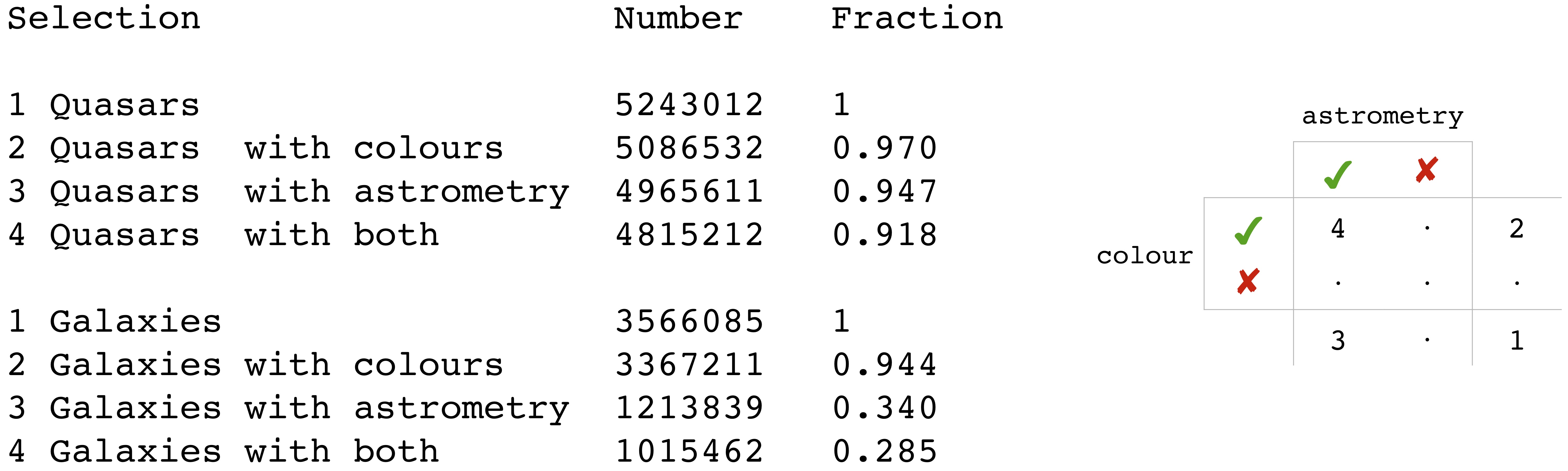
Classes are assigned (i.e. sources classified) by selecting all sources with a class probability above some threshold. The number of sources obtained for each class when adopting a threshold of 0.5 is show in Table 11.16. Figure 11.10 shows how many of these sources have colours and/or parallaxes/proper motions, for those sources with Combmod probabilities above 0.5 for the quasar and galaxy classes. We see that while most sources have BP/RP colours, most of those with higher galaxy probabilities do not have parallaxes/proper motions. In such cases there would have been no Allosmod results and so the classification is based only on the Specmod results, i.e. only on the BP/RP spectrum.
To assess the performance of DSC, we applied it to a validation set of sources of known class. For this to be meaningful, these classes should be consistent with the class definitions in DSC, and we achieve this optimally with four of the five classes by using a random subset of the superset from which the train/test data were drawn. The exception to this is physical binary stars: Because these were synthesized from Gaia data, they do not appear in the Gaia catalogue. For this class we instead use binaries identified in LAMOST-DR5 by Xiang et al. (2019). Note that this set itself does not have a very high purity, even when we limit it to high signal-to-noise ratio data. After crossmatching this to Gaia DR3 and retaining only sources with phot_bp_n_obs and phot_rp_n_obs equal to or greater than 5, we had 332 448 sources. Due to this mismatch between the class definitions in the training data and the validation data, we do not expect good apparent performance on binaries.
Taking the DSC probabilities on the validation data, we assign each source to that class which achieve the largest probability that is also greater than 0.5. If no probability is above 0.5 it remains unclassified. This is done separately for Specmod, Allosmod, and Combmod. Once we have these classifications we can construct the usual confusion matrix, and we summarize this using the completeness and purity of each class, as described in Bailer-Jones et al. (2019). As a reminder, the completeness is the fraction of true positives among all trues, and the purity is the fraction of true positives among all positives. However, we must then make an important adjustment to the confusion matrix: Because the class fractions in the validation set are not representative of what they are in Gaia, an unadjusted computation of the purity would give incorrect results. Specifically, stars are far less common in the validation data than they are in a random sample of Gaia data, meaning that there are far too few potential contaminants to the other classes in the validation data than in reality. This would lead to a significant overestimation of the purities. We can easily adjust the confusion matrix to accommodate this, however. As explained in section 3.4 (in particular equation 4) of Bailer-Jones et al. (2019), we can modify the confusion matrix so that the validation set effectively has class fractions equal to the class prior. This makes our purity results appropriate for any randomly selected sample of Gaia sources. Note that this correction is independent of the fact that DSC probabilities are already posterior probabilities that take into account this class prior. So to get meaningful estimates of performance we must both produce correct posterior probabilities using the class prior, and adjust the confusion matrix to reflect the same class prior.
If one wanted to assess the performance on some non-random selection of Gaia data, e.g. just brighter sources, then one could adjust the confusion matrix in the same way but using a different class prior that is more appropriate for that selection. In that case one should also adjust the DSC posterior probabilities (before assigning classes, of course) to take into account this new prior (see Section 11.3.2). We do this later in this section for low and high latitude sources.
| Specmod | Allosmod | Combmod | Spec&Allos | |||||
| compl. | purity | compl. | purity | compl. | purity | compl. | purity | |
| quasar | 0.409 | 0.248 | 0.838 | 0.408 | 0.916 | 0.240 | 0.384 | 0.621 |
| galaxy | 0.831 | 0.402 | 0.924 | 0.298 | 0.936 | 0.219 | 0.826 | 0.638 |
| star | 0.998 | 0.989 | 0.998 | 1.000 | 0.996 | 0.990 | – | – |
| white dwarf | 0.491 | 0.158 | – | – | 0.432 | 0.250 | – | – |
| binary | 0.002 | 0.096 | – | – | 0.002 | 0.075 | – | – |
| quasar, | 0.409 | 0.442 | 0.881 | 0.603 | 0.935 | 0.412 | 0.393 | 0.786 |
| galaxy, | 0.830 | 0.648 | 0.928 | 0.461 | 0.938 | 0.409 | 0.827 | 0.817 |
Table 11.17 shows the completeness and purity for the various classes and classifiers. This shows rather modest purities and completeness or all classes except star. This is the performance we expect for sources selected at random from the entire Gaia dataset that has complete data for Specmod and Allosmod. It accommodates the rareness of all these classes, as specified by the class prior (Section 11.3.2), both in the probabilities and in application data set. This gives a lower limit on the purities, as it includes many faint sources with low quality data. Due to the dominance of single stars in Gaia, we are not really interested in the performance on the star class. Indeed, it is trivial to get an excellent single-star classifier: just call everything a single star and your classifier has 99.9% completeness and 99.9% purity.
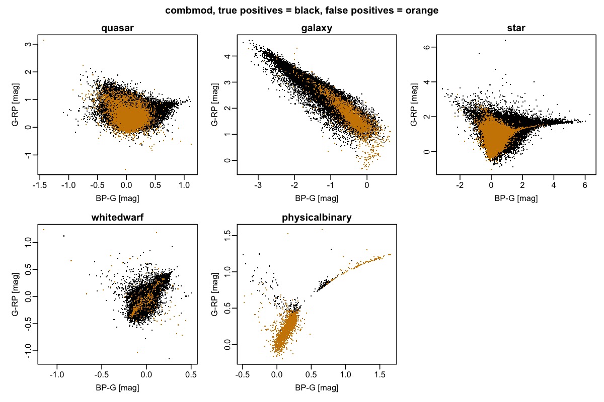
Figure 11.11 gives some idea of where the contaminants – the false positives – lie in colour space in relation to the true positives. The relative number of objects in each panel is not relevant, of course, as it simply reflects the class fractions in the validation set. In reality, a random sample of Gaia objects would be dominated by stars, so we would see far fewer false positives in the star panel, and far more in the other panels.
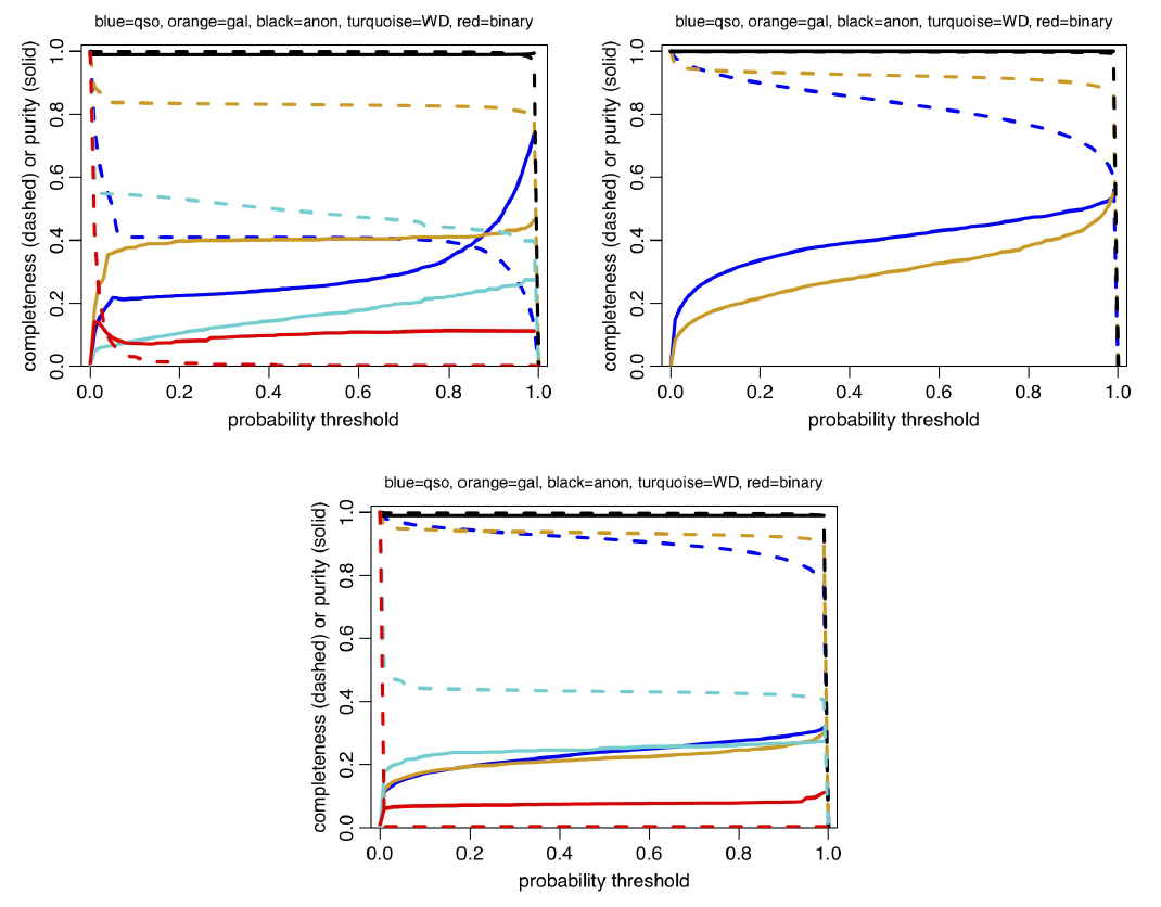
Figure 11.12 shows how the completeness and purity vary as a function of the posterior probability threshold used to build a sample. For Specmod the completenesses and purities vary little over a wide range of intermediate probability thresholds. This indicates that the Specmod posterior probabilities tend to be rather extreme (near to 0 or 1), which may be related to the fact that ExtraTrees classifiers do not really provide probabilities. Allosmod shows more variation, consistent with its likelihood modelling approach, and this is reflected to some degree also in Combmod. We see, for example, that if we raise the Combmod quasar classification threshold to 0.9 we would achieve a global purity of 0.6.
If we select a sample according to posterior probabilities above some value , we might expect a fraction of order of this sample to be contaminants (although the actual expectation depends on the distribution of the probabilities). However, the probabilities may not be perfectly calibrated, especially not from Specmod (and therefore Combmod), as ExtraTrees do not model the data distribution (unlike the GMMs of Allosmod). In principle, though, by knowing the confusion matrix we can compute the true class fraction in a sample given the measured class fraction, as explained in appendix B of Bailer-Jones et al. (2019).
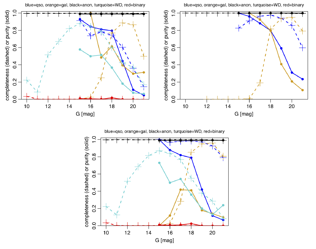
The purity and completeness of samples varies significantly according to how the sample is selected, e.g. magnitude or Galactic latitude range. The variation with magnitude is shown in Figure 11.13 when using a probability threshold of 0.5. (A plot for 0.99 can be found in Bailer-Jones 2021.) This is shown using the same global class prior in all magnitude bins (but the adjustment of the confusion matrix is done for the actual sample in each magnitude bin). Really we should vary the class prior as a function of magnitude, as we expect fewer extragalactic objects at bright magnitudes, for example.
We have explored the impact of such a prior adjustment on the performance for high and low latitude objects, where we define the former as those with , or , and the latter as those with . The fraction of extragalactic objects in Gaia is larger at high latitudes because (a) there is a smaller number of stars per unit area (compared to the sky average), on account of fewer disk stars and (b) more extragalactic objects per unit area are visible, on account of the reduced foreground extinction. Both of these increase the prior probability of a source being extragalactic and so this needs to be reflected in the computation of the posterior (and in the confusion matrix). We can easily accommodate (a) by counting the fraction of all sources (that are classified by DSC) at high and low latitudes, because almost all sources are stars. (b) is harder to account for, so we ignore it here and assume that true extragalactic objects in Gaia are uniformly distributed over the sky. Under these assumptions we find that the fraction of extragalactic sources at high latitudes is 2.7 times larger than the sky average. We therefore increase the class prior for quasars and galaxies by this factor and recompute the posteriors and the confusion matrix (again adjusting the latter for the actual sample in order to reflect the new prior). Specifically, we adopt a prior probability for quasars of (cf. globally), and a prior probability for galaxies of of (cf. globally). For the Combmod classifier, the quasar and galaxy purities are now both increased to 0.41, compared to around 0.22 globally (see Table 11.17). In other words, the expected contamination for a sample selected by maximum probability is reduced by a factor of two by avoiding the Galactic plane. The improvement is even larger for the Specmod and Allosmod classifiers, as can be seen in Table 11.17, and is even better still when we require both Specmod and Allosmod to give probabilities larger than 0.5 after the posteriors have been recomputed (last two columns of that table): the purities of the quasar and galaxy samples are now around 0.8. In all cases the completenesses hardly change. In reality the improvement in purity would be even more, because we have neglected aspect (b) mentioned above. The message is clear: limiting the sample to higher Galactic latitudes give much purer samples, with no change in completeness. Clearly, if we were willing and able to push the prior for extragalactic objects higher, we would get even higher purities. Of course, the contamination of the low latitude sample is larger than the sky average: we find the fraction of extragalactic sources here to be 3.5 times smaller, with the consequence that the purities in Combmod then drop to less than 0.1.
It is important to realise that these purity and completeness measures refer only to the types of object in the validation set. For extragalactic objects, this means objects classified as such by SDSS using the SDSS spectra. The overall population of extragalactic objects classified by DSC is of course broader than this, so the completeness and purity on other subsets of extragalactic objects could differ.
Uses and limitations
The DSC class probabilities are provided primarily to help users identify quasars and galaxies. Users can classify objects by selecting objects that have class probabilities above some freely-definable threshold (see Figure 11.12). For convenience we provide two class labels for the quasar and galaxy classes in the qso_candidates and galaxy_candidates tables corresponding to thresholds of 0.5 (see Section 11.3.2). In both tables the type classlabel_dsc_joint provides samples with larger purities, at the cost of lower completeness, as can be seen in Table 11.17. As mentioned above, even higher purities for quasars and galaxies can be obtained by selecting brighter and/or higher latitude objects.
The user must bear in mind that the classes are defined by the training data, and may be narrower definitions than one expects. Care must therefore be taken when comparing results to other catalogues. For example, the set of quasars used to define the CRF3 in Gaia explicitly removes sources that have have anomalously large parallaxes or proper motions, whereas we used these very anomalies in DSC to help with the classification.
While Specmod (and Combmod) produces class probabilities for five classes, its performance on binary stars and white dwarfs is generally poor. Binary star are difficult to distinguish from single stars using the data available for DSC. The actual performance on binaries as defined by the training set may be better than what we report on the validation data, however, due to the mismatch in the class definitions. The probabilities for these two classes are provided only in the astrophysical parameter tables and we recommend they are not used for building samples. The user could ignore these classes by adding their probabilities to ”star” to produce a ”non-extragalactic” class. We hope to improve the performance on these classes in Gaia DR4.
Performance on quasars and galaxies is reasonable when we consider how rare these objects are: assumed to be 1 in 1000 and 1 in 5000 respectively. We remind the reader that the probabilities provided are posterior probabilities that accommodate this, and so are appropriate for objects picked at random from Gaia using no other information.
The posterior probabilities provided of course depend on our choice of priors, and these are not easy to define accurately due to the unknown true population of the classes, plus the difficulty of calibrating Gaia’s selection function. Nonetheless, as any reasonable prior is very far from uniform, it is important that we adopt something roughly appropriate. Failure to do so gives both better apparent performance yet worse actual performance (Bailer-Jones et al. 2019). Users can easily adjust the DSC output probabilities to reflect other priors (see Section 11.3.2). We encourage users to think carefully about the appropriate prior for their use cases. For example, if one limits the selection a priori in some way, e.g. in magnitude, colour, or sky position, this affects the priors, potentially significantly, and therefore the expected completeness and purity (as we see in Table 11.17).
Better performance could be achieved by adding non-Gaia data, such as infrared photometry, but this was beyond the scope of the work for Gaia DR3. One of the goals of our work is to provide Gaia-only probabilities. It should be easy to combine these with probabilistic classification results from other surveys. When doing this, one must be careful to ensure that the prior is not counted more than once (see Section 11.3.2).