6.4.8 Single-transit analysis (STA)

Figure 6.7 presents a flowchart of the STA chain. The main inputs to the chain are the wavelength-calibrated, normalized observed spectra and the stellar parameters of the synthetic spectrum, as determined by CombineTemplate (Section 6.4.7). From the latter, the module GenerateTemplate (Section 6.4.8) produces a template; this template is normalized in the same way as the observed spectra (cf. Section 6.4.5).

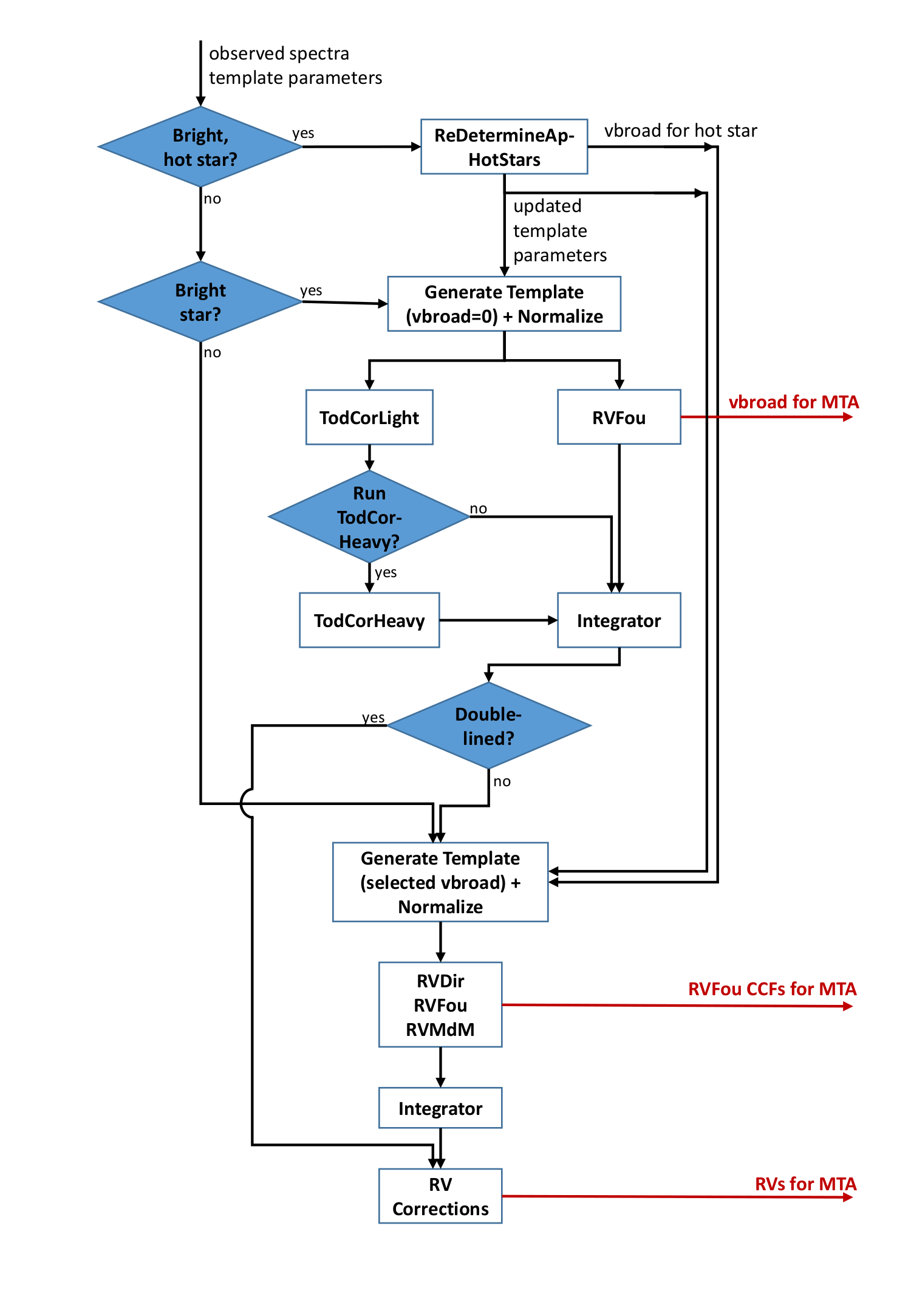
For the hotter stars, the selected synthetic spectrum does not always provide a good template for the observed spectra. In ReDetermineApHotStars, a better template is chosen, and the fields rv_template_teff, rv_template_logg, and rv_template_fe_h are updated. The required vbroad is also determined. It must be stressed that these template parameters do not necessarily represent the best astrophysical parameters for the star; they only represent the choice of the template that has been used to determine the radial and vbroad velocity. Details about the handling of hot stars are in given in Blomme et al. (2023).

For the brighter stars, the epoch vbroad is determined as detailed in Section 6.4.8.

To find and analyse possible double-lined spectra, STA uses a hybrid method (two-dimensional cross-correlation as proposed by Zucker and Mazeh (1994), followed by ${\chi }^2$ minimisation) designed so that it delivers not only the respective Doppler shifts and the brightness ratio of the presumed components, but also an estimate of their vbroad velocity and an uncertainty estimate for all values returned. Additionally, the algorithm fits a single-lined model to the same data and applies an F-test on the ${\chi }^2$ values to decide whether it should in fact be rejected in favour of the double-lined one. Since there is no a priori information on the nature of a presumed secondary component, many possibilities need to be considered. To reduce the resulting computational load, first a simplified version of the algorithm is applied to each observed spectrum. This is implemented by the module TodCorLight which assumes that both components have the same spectral type and rotational broadening and which sets a relatively low threshold in the F-test. Only the spectra which then emerge as suspected multiple are subsequently handled by the module TodCorHeavy which explores other spectral types and which rejects the single-lined model only with 99.9 % confidence. Both modules are described in more detail in Section 7.5 of Sartoretti et al. (2018). The following improvements are implemented in DR3:

• •

  different templates are used for the two components (while a single template was used in DR2);

• •

  the limits within which the binary model is accepted are extended and are:

  • –

  • –

    brightnessRatio $>0.2$

  • –

    $G_{\mathrm{RVS}}^{\mathrm{ext}}\le 11$ mag.

The two component radial velocities are then used to compute the orbital solution as described in Section 7.5. More description of the SB2 detection and related orbital solutions is provided in Damerdji et al. (2022).

Next, for all stars handled by STA a default epoch vbroad value is selected that is used to broaden the template before comparing it to the observed spectra. For the coolest stars ($\log T_{\mathrm{eff}}\le 3.8$), vbroad $=0$ $\mathrm{km}{\mathrm{s}}^{-1}$, for the hotter ones ($\log T_{\mathrm{eff}}\ge 3.9$) vbroad $=100$ $\mathrm{km}{\mathrm{s}}^{-1}$, and a linear transition (as as function of $\log T_{\mathrm{eff}}$) is used in between. If vbroad has been determined by ReDetermineApHotStars, then that value takes precedence.

The actual Doppler-shift measurement follows a multi-method strategy (David et al. 2014) involving standard cross-correlation using Fourier transform, Pearson correlation, and a minimum distance method, implemented respectively by the modules RVFou, RVDir, and RVMDM. The methods differ essentially by the choice of a C-function and by the algorithm for centroiding the C-function’s extremum. In principle each module produces a single Doppler-shift value per transit, along with an estimate of the internal uncertainty; these values generally differ somewhat because the effects of noise depend on the method.

The module Integrator combines the above results for storage in the main database, taking account of the several flags (cf. Section 6.4.8) which may have been set in previous processing steps. If the single-lined model was not rejected, the median of the radial velocities obtained by the modules RVFou, RVDir, and RVMDM is stored as the Spectroscopic Radial Velocity (SRV), the corresponding internal uncertainties being propagated accordingly. Otherwise these measurements are ignored and the results from TodCorHeavy are stored instead. All STA radial velocity values are in the Gaia-centric frame.

Finally, some corrections to the radial velocities are applied, as detailed in Section 6.4.8.

The spectra from the three CCDs in a transit may exhibit small differences in wavelength zero point, wavelength range, and sampling which means that they cannot be simply summed if one needs to combine their information. Therefore all modules that determine radial velocities expect three spectra in a transit (though they can handle the case where one or two of these are missing). They first perform their measurements on each spectrum separately, storing the C-functions used in that process; subsequently they combine these C-functions on a common velocity grid (see Sartoretti et al. 2018) to use the information from the whole transit. Only the latter results are propagated along the STA chain while the single-CCD measurements are used for internal diagnostic purposes.

The synthetic spectrum that is associated with each RVS spectrum is selected among the synthetic spectra of the auxiliary spectral library (Section 6.2.3). The selection is based on the weighted minimum distance between the atmospheric parameters that are associated with the star and those associated with the synthetic spectrum. The distance to minimise is:

where $T_{\mathrm{eff}}$, $\log g$, and $[\mathrm{Fe}/\mathrm{H}]$ are associated with the star and, $T_{\mathrm{eff}}^{\mathrm{tpl}}$, $\log g^{\mathrm{tpl}}$ and $[\mathrm{Fe}/\mathrm{H}]$ ${}^{\mathrm{tpl}}$ with the synthetic spectrum; $T_{\mathrm{eff}}$ is in K. The weights of 100, 3, and 2 are an ad hoc estimate to give more weight to a difference in $T_{\mathrm{eff}}$ (on which the morphology of the spectrum depends most) than in $\log g$ or $[\mathrm{Fe}/\mathrm{H}]$.

GenerateTemplate can convolve the synthetic spectrum with a rotational profile (Gray 2005). However, when the purpose is to determine the epoch vbroad (for sufficiently bright stars), no such convolution is applied, and it is left to the RVFou module to apply the broadening during its search for the best vbroad value. When determining the radial velocity, GenerateTemplate does apply the broadening, as discussed in Section 6.4.8.

Next, the spectrum is convolved with the instrumental profile (LSF-AL, Section 6.3.4). This instrumental profile is different for each of the three spectra of a single transit. The resulting spectrum is resampled to a wavelength step of 0.00747 nm, which is 10 times finer than the nominal resolution element of the RVS. The template is thus oversampled to facilitate the subsequent shifting–, convolution– and resampling operations performed by the STA modules.

The wavelength range of the template is 843–873 nm. This is larger than the 846–870 nm range of the observed spectrum to ensure that the template, shifted within the RVS velocity range of $\pm 1000$ $\mathrm{km}{\mathrm{s}}^{-1}$, can be resampled on the wavelength grid of the object spectrum without loss.

The template is normalized in the same way as the observed spectra (Section 6.4.5).

For each transit of a sufficiently bright star ($G_{\mathrm{RVS}}$ $\le 12$), RVFou explores a predefined grid of vbroad values. For each value, it convolves the non-broadened template with the corresponding rotation profile, then cross-correlates the broadened template with the observed spectrum from each CCD, and combines the resulting CCFs (Section 6.4.8). The peak heights of the combined CCF define a function of the vbroad values; the vbroad value corresponding to the maximum of that function is the estimate for the transit at hand. The transit values of vbroad are passed on to MTA, which in turn determines the vbroad value for the source (Section 6.4.9). More details and the validation of this method are given by Frémat et al. (2023).

The characteristic discussed here is named vbroad in the catalogue and not $v\sin i$. The reason for this choice is that, while the rotational profile (Gray 2005) is used to measure line broadening, there may be other factors causing the broadening of the observed spectral lines (e.g., macroturbulence, residual instrumental effects, spectrum mismatch, the presence of an undetected secondary component, etc.) so that the measured value does not represent ‘pure rotation’ but possibly a mix of broadening mechanisms. Among these, of course, rotation will mostly be dominant.

In the course of STA, several boolean flags are used to signal particular problems with, or characteristics of, each transit:

• •

  isValid (default=1) is set to 0 by any of the modules mentioned above, if a computational problem is encountered which renders the output of the module meaningless (e.g., division by zero, lack of convergence in an iteration, etc.).

• •

  isAmbiguous (default=0) is set to 1 by the modules RVDir, RVFou, RVMDM, or TodCorLight, to indicate that the single-CCD radial velocity values from a given transit are not consistent between the CCDs, in view of their uncertainty. Mostly this is due to the fact that the single-CCD spectra are too noisy to allow a Doppler-shift measurement whose uncertainty is correctly described by the internal uncertainty estimate, but there may be several other reasons, e.g., a residual blemish in the data, strong template mismatch, etc. If the reason for ambiguity is merely noise, the MTA radial_velocity estimation method used for the faint stars (rv_method_used=2) may yet allow a meaningful radial velocity measurement (Section 6.4.9).

• •

  suspectedMultiple (default=0) is set to 1 by TodCorLight if a double-lined model fits the observed spectrum significantly better than a single-lined one.

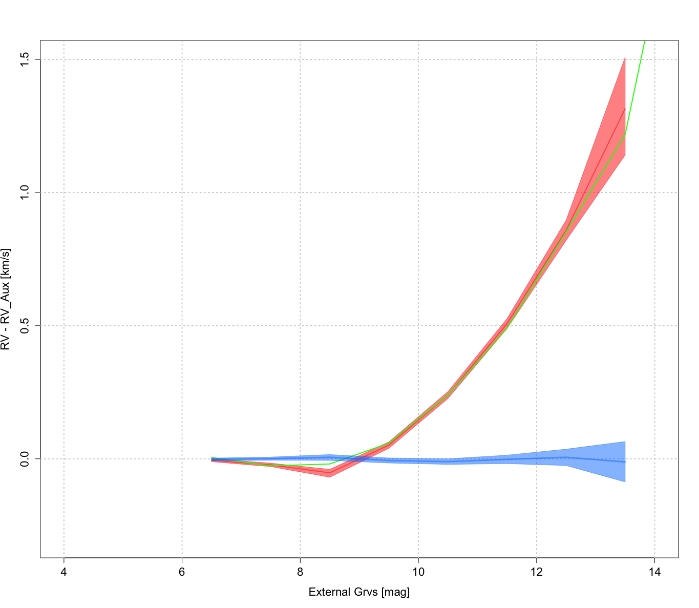
By comparing the radial velocities determined by STA with values from the literature, an offset was discovered that depends on both magnitude and time. Figure 6.8 shows an example of the magnitude-dependent offset for CCD row 4 and for a low straylight background. The offsets ($V_{\mathrm{rad}}$ ${}_{Gaia}$ - $V_{\mathrm{rad}}$ ${}_{\mathrm{literature}}$) for each individual star were grouped in bins of $G_{\mathrm{RVS}}$ magnitude, and the median of each bin was determined. A polynomial was then fit against these medians as a function of $G_{\mathrm{RVS}}$. This polynomial was then used to correct the offset of all STA determined radial velocities. While this procedure does not elimate the magnitude-dependent offset on an individual star basis, it does so on the median (as a function of the $G_{\mathrm{RVS}}$ bins). This can be seen on Figure 6.8, where the corrected radial velocities offsets from the literature values are shown in blue colour. The coefficients of these correcting polynomials depend on CCD row (Section 1.1.3) and straylight background level (Section 6.4.3).

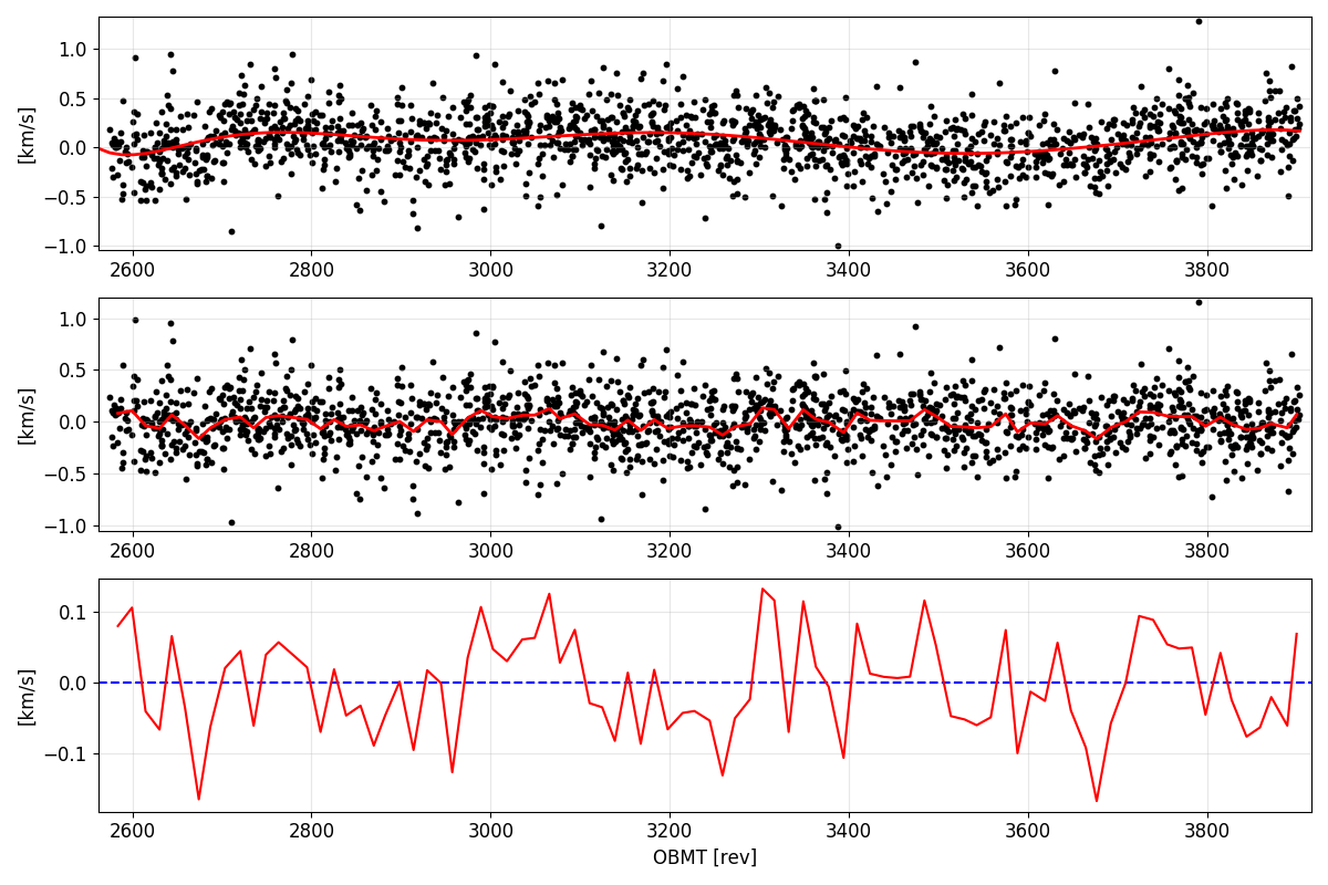
An example of the offset with time is shown in Figure 6.9. Polynomial fits (or, in some cases, a simple median) are used to correct for this time-dependent offset, in a similar way as for the magnitude-dependent offset. The coefficients of these fits depend on trending epoch (Section 6.2.1), field of view and CCD row.

A comparison between the intrinsic radial velocity uncertainty derived by STA and the dispersion of the epoch radial velocities showed they are inconsistent. The intrinsic radial velocity uncertainties were therefore corrected using polynomials depending on $G_{\mathrm{RVS}}^{\mathrm{ext}}$ (Section 6.1.2) and $T_{\mathrm{eff}}$ (Section 6.2.3) in a similar procedure as for the radial velocity corrections described above. The polynomials are valid for $G_{\mathrm{RVS}}^{\mathrm{ext}}$ between 3 and 12 mag and log $T_{\mathrm{eff}}$ $\ge$ 3.5. Outside the validity area the values at the border were taken (and this explains the systematic underestimation of the intrinsic errors for the faint stars shown in Figure 6.13).

For most stars, these radial velocity uncertainties are not part of Gaia DR3. The exception is the radial velocity information for some 2000 Cepheid and RR Lyrae stars published in the table vari_epoch_radial_velocity and described in Clementini et al. (2023) and in Section 10.5 and Section 10.11.