6.4.4 Calibration
In the Calibration pipeline the spectra of the potential calibrators (non-blended transits of the stars brighter than 10) are processed in order to calibrate the RVS instrument and to produce the calibration models described in Section 6.3. The calibration models (called GenericTrending) are then applied to all the RVS spectra in FullExtraction. This pipeline includes various steps:
-
•
Preprocessing: This is the first step, mostly technical, where the information contained in the input data (Section 6.2) is treated and reformatted into the objects used by the downstream steps of the pipeline. The filters on the input data are also applied. The input selection includes the spectra of the stars brighter than mag and with rectangular windows. The rectangular-truncated windows are also included. In fact, some bright stars produce nearby spurious sources and have a truncated but rectangular window, their spectra are re-blended when the missing part of their window is found among the pipeline inputs.
The astrometric information (AGIS coordinates, OGA3 and the Gaia Ephemeris) is used to associate to each sample of the spectrum the FoV coordinates of the source at the time when the sample crosses the CCD fiducial line, and the barycentric velocity correction (Section 3.4.6) is associated with each spectrum.
The transits of potential contaminants are identified: these are the transits of the potential contaminant-sources selected in SourceInit, brighter than and not having an RVS window. The transits having a relatively bright and nearby contaminant are then removed during the Calibration preparation step.
-
•
Calibration Preparation: This step is in charge of selecting the potential calibrators, to clean their spectra and to apply the initial calibration model (Section 6.2.2). See Section 6 of Sartoretti et al. (2018) for more details.
-
–
Bias and bias non-uniformity is first removed using appropriate calibration coefficients (see Section 6.3.1).
-
–
Saturated samples (65 535 ADU) are flagged. The spectra presenting a saturated sample are later removed from the pipeline.
-
–
The fixed CCD gain that was measured on ground, is applied.
-
–
The dark current that was measured on ground, is subtracted (see Section 6.3.2).
-
–
The straylight background is removed by subtracting the flux from the cell in the RVS straylight map that corresponds to the processing window’s position, time and pixel sampling. The spectra with a total negative flux resulting from a too high-background subtraction are filtered from the pipeline, and so are the spectra for which the background was higher than 100 electrons pixel s.
-
–
The flux loss outside the window is estimated using the initial LSF-AC calibration model.
-
–
Windows that contain any columns from the cosmetic defect list (see Section 6.3.2) are flagged and filtered from the pipeline.
-
–
Windows having a nearby relatively bright contaminant (i.e. a source with no RVS window and with a magnitude brighter than the target source magnitude + 3 mag, and within a relevant contamination area around the target source of about 2500 AL x 20 AC pixels), are flagged and filtered from the pipeline.
-
–
Cosmic rays are removed from both 2D and 1D windows. If pixels are saturated due to cosmic rays and the cosmic ray is successfully removed, the saturation flag is turned off and the window can proceed in the pipeline, otherwise it is filtered from the pipeline. The spectra presenting a saturated sample are removed from the pipeline.
-
–
2D windows are optimally collapsed into 1D spectra.
-
–
The initial wavelength coefficients are applied to the field angles and wavelength range is cut to 846–870 nm to avoid the RVS filter wings.
-
–
The RVS filter response that was measured on ground, is removed.
-
–
The spectra are normalised to their pseudo-continuum using a -degree polynomial fitting. The stellar lines are iteratively rejected using a sigma-clipping with interval .
-
–
Detect and flag the emission-line spectra (these spectra are not used in calibration).
- –
-
–
Select the reference stars for each calibration task: The wavelength calibration module needs high SNR spectra presenting deep absorption lines. Therefore the calibrators are selected based on their magnitude ( mag) and on their atmospheric parameters ( K). Figure 6.6 shows an example of a wavelength calibration star spectrum.
The calibration of the LSF-AC profile and peak position requires very bright stars ( mag) with 2D window; the LSF-AL calibration requires the RVS spectra of the stars for which the ground-based spectrum is available (Section 6.2.3) and with mag. The calibration of the zero point requires the RVS spectra of the stars for which the reference magnitude is available (Section 6.2.3) and with mag.
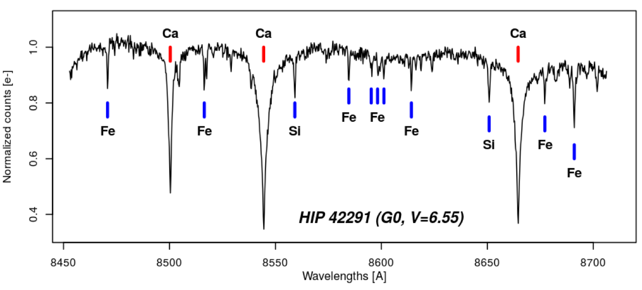
Figure 6.6: The RVS spectrum of a bright star used in wavelength calibration. The spectrum is dominated by the three Ca II lines. Some of the iron, and silicon absorption lines are also indicated. The wavelength range used extends from 846 to 870 nm, with a sample size of about 0.0245 nm corresponding to about 8.6 . Figure from Sartoretti et al. (2018).
-
–
-
•
Calibration and trending
The wavelength calibration coefficients, the LSF-AL profile, the LSF-AC profile and peak position coefficients and the zero point, are derived for every calibration unit, in each trending epoch, according to the calibration models (see Section 6.3). The duration of a calibration unit is 30 hours in wavelength and zero point calibrations and it is 1 hour in the LSF-AL calibration to ensure that most calibration units include enough RVS observations of auxiliary data, which the calibration requires. The calibration unit is about 0.5 hours for the LSF-AC profile and peak position, where the variations are rapid due to the AC motion of the sources.
The trending consists of fitting a function with respect to time to each calibration coefficient (see Figure 6.12 for an example of trending). To have a trend function with respect to time means that it does not matter if the calibration in any one calibration unit does not produce coefficients, as long as this is not too often. Moreover, fitting a function with outlier rejection allows the trend functions to be more robust against noise and outliers.