6.4.9 Multi-transit analysis (MTA)

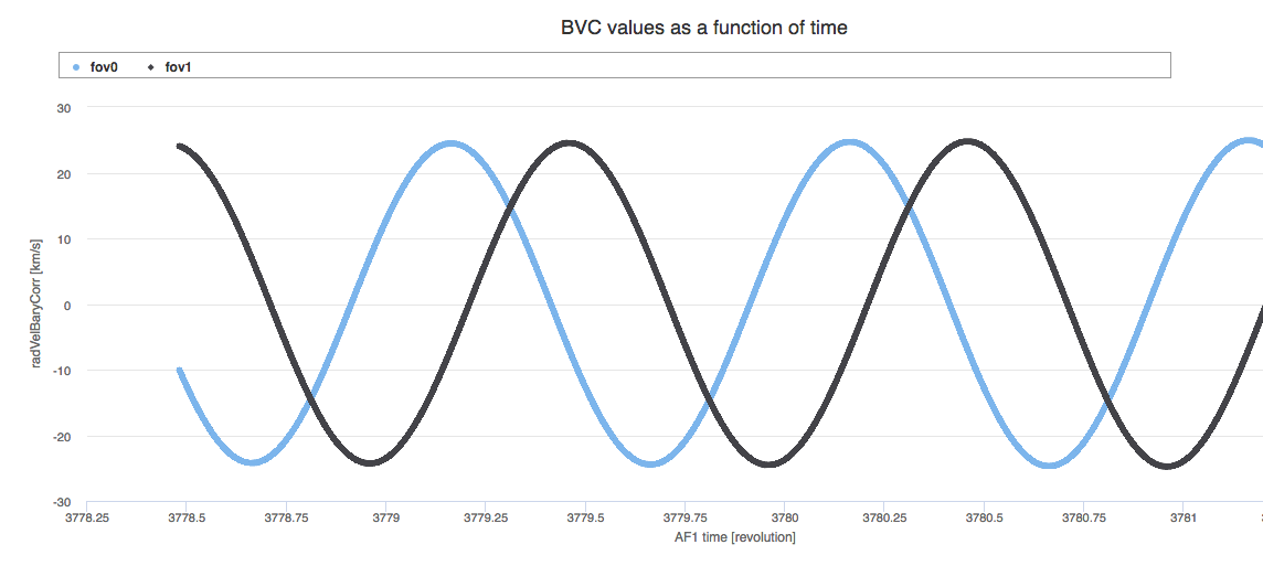
The STA Gaia-centric radial velocities are converted to barycentric by adding their barycentric radial velocity correction (Section 3.4.6), which can range from about $+30$ $\mathrm{km}{\mathrm{s}}^{-1}$ to $-30$ $\mathrm{km}{\mathrm{s}}^{-1}$ as a function of Gaia’s six hour revolution (Figure 6.10). The C-functions are shifted by the barycentric radial velocity correction and by the systematic offsets described in Section 6.4.8.

The multi-transit radial velocities (radial_velocity) are obtained in the two different ways (rv_method_used), depending on the magnitude grvs_mag of the star:

• •

  grvs_mag $\le 12$ mag the radial_velocity is the median of the single-transit barycentric radial velocities, and the error is the error on the median. For these bright stars, the single-transit radial velocities are expected to be precise and accurate enough, and the parameters rv_amplitude_robust, rv_chisq_pvalue, and rv_renormalised_gof are published.

• •

  grvs_mag $>12$ mag or no grvs_mag information, the radial_velocity is estimated using the multi-transit combined C-function. The epoch C-functions from the STA method RVFou are shifted by the barycentric velocity correction and by the systematic offsets, and then combined. The combined C-function is then used to obtain the radial velocity using the RVFou method. For a detailed description of RVFou, see Sartoretti et al. (2018, Section 7.2).

The uncertainty on the multi-transit radial velocities is estimated differently in the two methods and is provided in radial_velocity_error.

The multi-transit broadening velocity, vbroad, is the median of the single-transit measurements obtained in STA (Section 6.4.8), leaving aside the values obtained with deblended or re-blended spectra and those obtained before the decontamination at OBMT 1317. The uncertainty associated with vbroad is provided in vbroad_error and the number of single-transit measurements used in vbroad_nb_transits. The computation and validation of vbroad is described in detail in Frémat et al. (2023).

The multi-transit $G_{\mathrm{RVS}}$, grvs_mag, is the median of the single-transit $G_{\mathrm{RVS}}$ measurements obtained in FullExtraction (Section 6.4.5), leaving aside the values obtained with deblended spectra and those obtained with spectra having rectangular truncated windows. A consequence of this is that the stars having only blended transits do not have grvs_mag information published in DR3.

The single-transit $G_{\mathrm{RVS}}$ is the median of the $G_{\mathrm{RVS}}$ obtained in each of the three CCD calibrated spectra. For each CCD spectrum, the total flux (between 846 and 870 nm), is computed and corrected for the flux-loss outside the window. The flux in the bad samples is replaced with the median flux in the good samples. The $G_{\mathrm{RVS}}$ zero point corresponding to the time, the CCD and FoV of the spectrum is extracted from the calibration model (see Sartoretti et al. 2018, Section 5.5).

The uncertainty associated with grvs_mag is provided in grvs_mag_error and the number of single-transit measurements used in grvs_mag_nb_transits. The computation and validation of grvs_mag is described in detail in Sartoretti et al. (2023)

The mean spectra are available in the table rvs_mean_spectrum for the sources having the flag has_rvs set. They are the result of the combination of the RVS CCD spectra output from the FullExtraction pipeline (Section 6.4.5); there are in general 3 CCD spectra per transit. The cleaning and the calibration of the CCD spectra is described in detail in Sartoretti et al. (2018), the deblending in Seabroke et al. (2021, Section 2.5) and their validation in Seabroke et al. (2022).

The brightest RVS mean spectra are used by the atmospheric parameter pipeline (Chapter 11) to estimate the star atmospheric parameters and the abundances of some elements, and it was decided to publish about 1 million of them.

The cleaned and calibrated CCD spectra, before combination, are normalised to the pseudo-continuum and shifted to the rest frame. The normalisation of the M stars (presenting the TiO band) and of the too noisy spectra is done by simply scaling with a constant. The shift to the rest frame is done using the Gaia-centric single-transit radial velocities when rv_method_used=1, and using the multi-transit radial_velocity (with the barycentric velocity correction removed) when rv_method_used=2. The CCD spectra with detected artefacts in the fluxes (flagged ‘hasJumps’) are excluded from the combination.

Once normalised and shifted to the rest frame, the CCD spectra are interpolated to a common wavelength array (start $\lambda =846$ nm, $\mathrm{\Delta }\lambda =0.01$ nbBins=2401) and averaged, taking care of removing the bad samples, notably the samples saturated, affected by cosmic rays, or badly deblended. The fluxError associated with each sample of the combined spectrum is the error on the average. The signal to noise ratio rvs_spec_sig_to_noise is estimated as the median value of the ratio between fluxes[i] and fluxError[i]. Due to a different number of samples used, the fluxError[i] may vary within a single spectrum, this variation may be significant, especially at the spectra edges, when the number of transits combined is small.

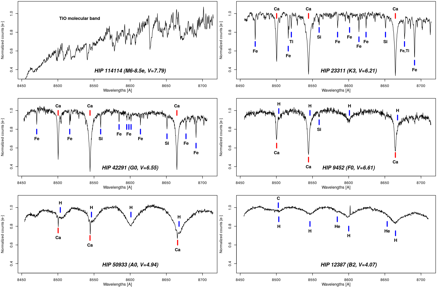
Some examples of RVS spectra of various spectral type bright stars are shown in Figure 6.11.

rvs_mean_spectrum can be extracted from the main archive up to a limit of 5000 sources at a time. For downloading more than 5000 sources at a time, it is possible to use a Python script (an example of such a script is given in the appendix of Seabroke et al. (2022)). Once you have made your query on has_rvs=t with fewer than 5000 sources, click on the DataLink icon on the right (two links of a chain). In the window that has popped up, in the Data release option, select Gaia DR3 and click on “Show Data”. This should show “RVS mean spectra (n)” in the list, where n is the number of sources with RVS mean spectra. Selecting “INDIVIDUAL” and clicking on the download icon next to “RVS mean spectra (n)” will create individual files in a separate folder within your usual downloading location, with one RVS mean spectrum per xml file. Selecting “COMBINED” provides a single xml file for download. The “INDIVIDUAL and “COMBINED” options provide the columns wavelength, flux, flux_error in a table format, while the other columns are stored in the header of the xml files. The “RAW” option provides all the columns as columns in a table, where flux and flux_error are arrays.