6.5.1 Verification
The verification of the results obtained in each processing step (Section 6.4) is done automatically via the Automated Verification workflows in charge of producing diagnostic plots which permit to verify the products of each processing pipeline.
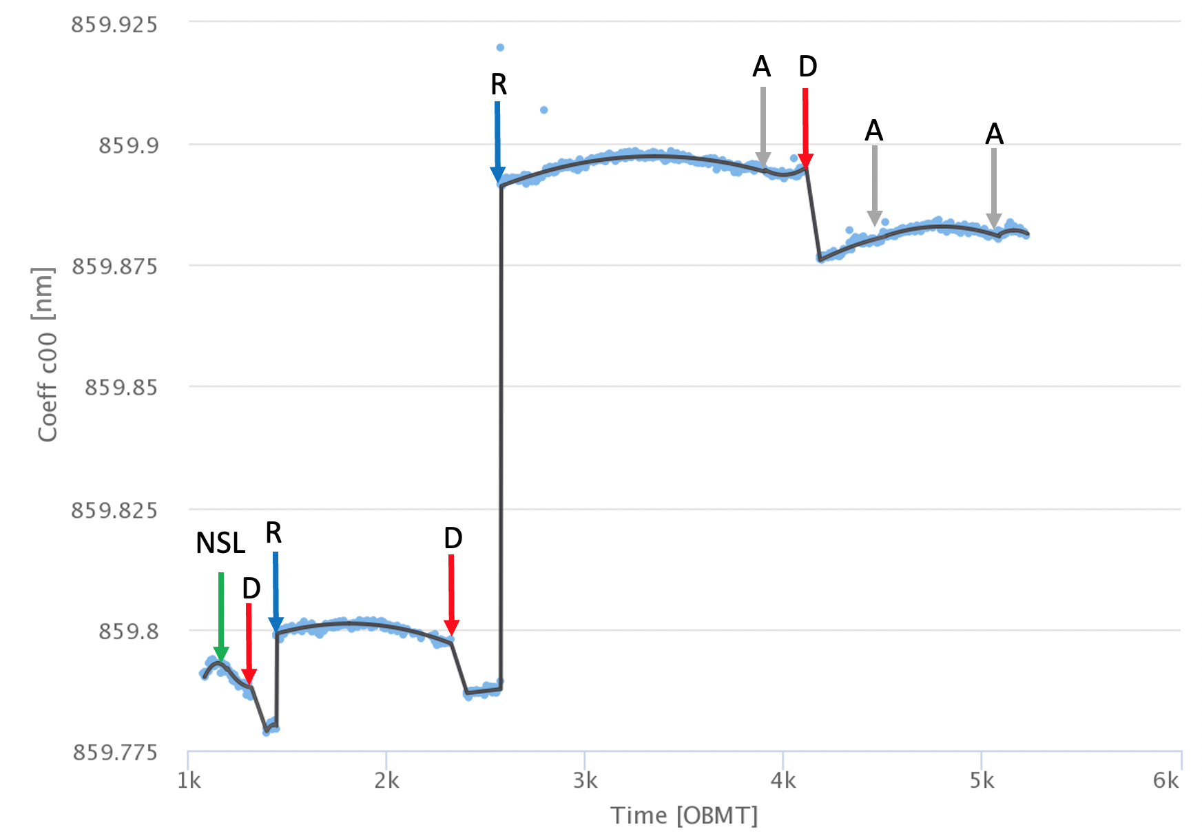
Some examples, among the many verification diagnostics, include the monitoring of the number of input and output data, of the properties of the spectra (like the window class, the blending status, etc.), of the number of invalid transits and of the invalidity reason. The electronic bias level, the total detection noise, and the barycentric velocity correction (Figure 6.10) are also monitored. In the Calibration pipeline, the number of the calibration stars and of the standard stars used in each calibration unit are monitored to verify they are in sufficient number and the trending plots of the calibration models obtained are provided for visual inspection (an example is in Figure 6.12).
The verification of the FullExtraction pipeline includes plotting of some of the spectra that have been rejected from the data flow because of bad quality (i.e. caused by one the rejection reasons in Section 6.4.5). The total number of spectra, with mag, that went successfully through FullExtraction is about 2 billion, about 30 % of them undergone deblending. The number of rejected spectra is approximately 855 million, the large majority (about 70 %) is rejected because requiring deblending but could not be deblended properly. Automated Verification also counts the number of cosmic rays and saturated samples detected and the number of spectra per various transit properties.
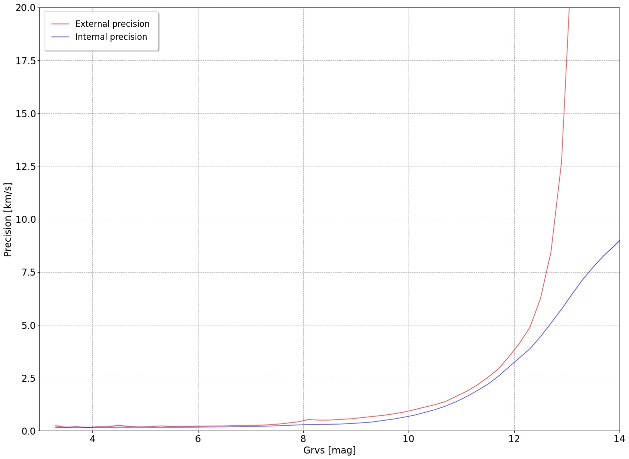
There are various automated diagnostics in charge of the verification of the STAMTA pipeline. Most of them rely on the comparison of the pipeline products with external ground-based reference data to estimate the accuracy and the external precision of the pipeline measurements as a function of grvs_mag and of the atmospheric parameters. For the radial velocities verification, the catalogues used are those listed in Table 6.3, together with the radial velocities of some open clusters (Soubiran et al. 2018a; Cantat-Gaudin et al. 2018, 2020). Despite the correction applied (see Section 6.4.8), the radial_velocities still present an overall small bias increasing with grvs_mag starting at about grvs_mag mag and reaching the value of about 300 at grvs_mag mag. Figure 6.13 shows the comparison of the external and internal precision for the epoch radial velocities. Some statistic information plots are also automatically produced, like the distribution of the star atmospheric parameters (Figure 6.3), or of the number of transits per star: the median number of transits of the stars having a radial_velocity is 17 and the average is 18. The good quality of the final radial velocity results is also an indirect proof of the correct behaviour of the upstream workflows.