6.1.2 Overview of the spectroscopic processing
The RVS spectroscopic processing pipeline is the result of the work of CU6 (Section 1.2.2): the scientific teams provided the scientific codes to DPCC (CNES), who integrated them in the SAGA (System of Accommodation of Gaia Algorithms) host framework. SAGA is developed by Thales. The RVS pipeline was run at DPCC (Section 1.3.5) on an Hadoop cluster with 2500 cores and 17 TB RAM. The processing took approximately 3 million hours CPU time and about 120 days real time, and needed 300 TB disk space.
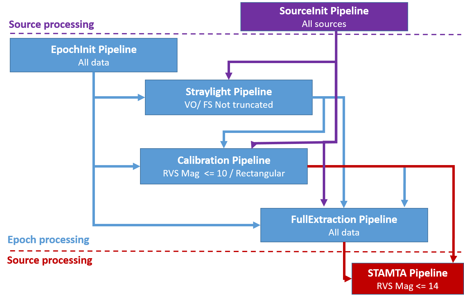
The technical design of the DR2 RVS pipeline was completely revised in order to make possible the treatment of many more data (2.8 billion of spectra in DR3 against 280 million in DR2) and to avoid the storage of voluminous intermediate data. The DR3 pipeline is composed of the 6 specialised pipelines shown in Figure 6.1.
New scientific functionalities introduced in the DR3 RVS pipeline
The main goal of the DR3 spectroscopic pipeline is to estimate the radial_velocity of as many stars as possible observed by the RVS and brighter than mag. This magnitude limit increases at each data release: it was mag in DR2, and it is expected to be mag in DR4. This is because at each data release the number of observations per source increases, and so does the expected signal to noise in the combined spectra, permitting to measure the radial_velocity of fainter stars. Listed here are the new scientific functionalities implemented in the pipeline which have permitted to accomplish the DR3 objectives.
-
•
Radial velocities of faint stars: The radial velocities of the faint stars (fainter than grvs_mag mag, but brighter than mag) are estimated. This is thanks to the implementation of rv_method_used=2 in the STAMTA pipeline (Section 6.4.6). For the sources fainter than grvs_mag mag, the radial_velocity is estimated using the combined epoch cross-correlation functions (C-function, Section 6.4.8) and not the epoch radial velocities, which are imprecise.
-
•
Straylight calibration (Section 6.4.3): the straylight map is estimated every 30 hours, and the spectra borders of the faint stars are also used, in addition to the Virtual Objects (VOs; Section 1.1.3). In DR2 a single straylight map was computed off-line using only the Ecliptic Poles Scanning Law (Section 1.1.4) data, and was used to process all the data. A better estimation of the straylight permits a better estimation of grvs_mag for the faint stars.
-
•
Deblending of the CCD spectra: the transit spectra contaminated by nearby sources with an RVS window are deblended and used to obtain the radial_velocity and the rvs_mean_spectrum of the source, while in DR2 they were removed from the pipeline. The deblending functionality permits to have a larger number of epoch spectra per source, increase the SNR of the combined CCF and estimate the radial velocity of the stars with fainter magnitude. It improves in part also the contamination problems shown by some rectangular truncated windows in DR2, reported by Boubert et al. (2019). The deblending algorithm is described in Seabroke et al. (2021), their Section 2.5.
-
•
Calibration of the Line Spread Function (LSF): The along-scan LSF (LSF-AL) profile, the across-scan LSF (LSF-AC) profile and peak position are calibrated (Section 6.3.4). The LSF-AL calibration has permitted to reduce the systematic shifts between the two FoVs which were present in the wavelength calibration zero point and reflected in the epoch radial velocities, while the LSF-AC and AC-Peak are needed by the deblending implementation, and by the estimation of the flux loss out of the window, which is taken into account in the computation of grvs_mag.
- •
-
•
Contamination from nearby sources without an RVS window: In DR2 the contamination from the sources without RVS window was not considered. In DR3, the contamination from sources without a RVS window and brighter than is taken into account in the following way. When the contaminant is in a relevant area around the target (about 2500x20 pixels) and the difference in magnitude with the target is 3 mag, the target CCD spectrum is removed from the pipeline.
-
•
Quality indicators based on the combined cross-correlation functions were developed and used in Post-processing (Section 6.5.2) to identify and flag as invalid spurious radial velocities.
-
•
Magnitude used for data selection: the selection of the data for the processing steps is done using the magnitude , obtained using and from DR2, and not anymore using the Initial Gaia Source List (IGSL) magnitude. When and are available the transformation used is (Gaia Collaboration et al. 2018a):
For - mag:
For mag: