10.2.3 Processing steps
Overview
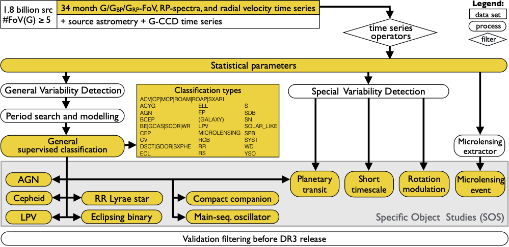
An overview of the variability processing is presented in Figure 10.1. Our application of time-series operators and a general selection of 5 FoV transits in the band selected 1.8 billion sources, which were processed through the different parts of the variability pipeline, as detailed in the following sections.
Initial time-series pre-processing
Definition of observation time
Observation times were expressed in units of Barycentric JD (in TCB) days, computed as follows:
-
1.
The observation time was converted from On-board Mission Time (OBMT) into Julian date in TCB (Temps Coordonnée Barycentrique).
-
2.
A correction was applied for the light-travel time to the Solar System barycentre, resulting in Barycentric Julian Date (BJD).
-
3.
Although the centroiding time accuracy of the individual CCD observations was (much) below 1 ms, the per-FoV observation times processed and published in Gaia DR3 were averaged over typically nine CCD observations, i.e., within a time interval of about 44 s.
Conversion from flux to magnitude
In the variability pipeline, magnitudes rather than fluxes were used in the various processing modules. To convert to magnitude, the zero-point magnitudes for , , and in the Vega system were used (Section 5.4.1).
Measurement filtering
The variability processing included several operators, which were applied to the time-series photometry. Typical time-series operators performed flux-to-magnitude conversion, outlier removal, and error cleaning on the input time series, to create derived (transformed and/or filtered) time series suitable for processing by subsequent algorithms. These time-series operators were chained in a hierarchy of derived time series, which were used as required by the scientific analyses, while ensuring that provenance was preserved.
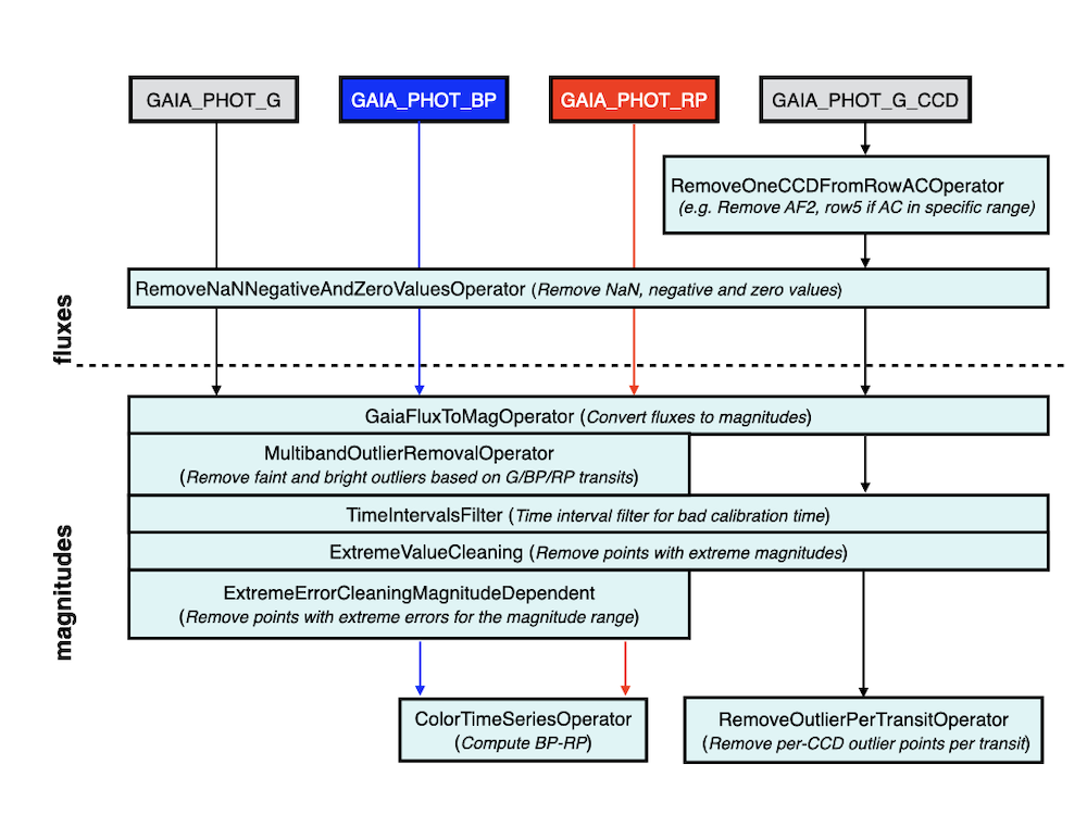
The following list of operators, whose hierarchy is illustrated in Figure 10.2, was applied sequentially to the input photometric time series:
-
1.
RemoveNaNNegativeAndZeroValuesOperator: it removes photometric transits that contain NaN, negative, or zero flux values.
-
2.
RemoveOneCCDFromRowAcOperator: it is designed to remove one CCD measurement (defined by its CCD number, between zero and nine, zero standing for the Sky Mapper and one to nine for the Astrometric Field CCDs) from each transit of per-CCD data whose measurements correspond to a certain CCD row and whose across-scan (AC) coordinate is outside a certain range (minimum AC=3, maximum AC=1990). It was motivated by the fact that the photometric calibration team reported problematic flux measurements for the second Astrometric Field (AF) CCD of row 5, when AC is greater than 1200. Hence, in Gaia DR3 this operator was tailored to remove the AF2 points for transits with CCD row=5 and AC coordinate .
-
3.
GaiaFluxToMagOperator: it converts fluxes to magnitudes by using the zero-point magnitudes in the Vega system (Section 5.4.1).
-
4.
MultibandOutlierRemovalOperator: this new operator in Gaia DR3 takes the advantage that , , and data are quasi-simultaneous and share the same transit_id. It removes data by identifying outliers in the different bands and takes into account the other bands in deciding whether the transit is a ‘real’ outlier to remove from a specific band, or not. The procedure followed by the operator is as follows:
-
(a)
In each band, a transit is flagged as a candidate outlier if the ratio
is above a threshold of three, where mag is the transit magnitude in a band, median(mag) is the median magnitude of all transits, and IQR(mag) the interquartile range of the input time series.
-
(b)
A sum is computed where each band with a flagged transit (candidate outlier) is counted as a unit with a positive or negative sign for an outlier that is brighter or fainter than the median magnitude, respectively (thus, the sum can range from to ). If the absolute value of the sum is and the outlier in the band has the same sign as the outlier in another band, candidates outliers are considered as non-outliers (thus outliers in and but not in are considered as real outliers). If there is a single outlier candidate in one band but without measurements in the other bands, the point is kept as non-outlier.
-
(c)
If only one band has a candidate outlier and measurements exist (in the same transit) in the other bands, the threshold for candidate outlier is reduced to one and the same procedure is followed as described in the previous item. Additionally, if there are outlier candidates and one of them has a different sign, only the outlier with a different sign from the one in the band is flagged as real outlier.
-
(d)
For the remaining candidate outliers, the iqrMedianMag in and/or are divided by the one in . If the ratio is above five, the outlier in and/or is considered as a real outlier. The same is repeated employing the lower iqrMedianMag threshold of one.
-
(e)
Finally, the following ratio
is used with a threshold of 20 for and 10 for and to flag transits with outlying errors. These conditions were applied to each band independently of the other bands and they were not used if the transit was initially a candidate outlier (in magnitude) that was eventually ruled as non-outlier.
This operator decreased the number of outliers considerably, while properly keeping the ones due to real astrophysical properties (e.g., flares, eclipses), but spurious outliers still remained (and can be particularly significant in and ). Moreover, this operator is not suitable to detect ‘impostor’ transits from nearby sources (mistakenly assigned to the incorrect source), as their bright or faint deviations are typically consistent in all bands.
-
(a)
-
5.
TimeIntervalFilter: it removed measurements in each individual band for OBMT in specific time ranges. Problematic observation times were identified based on a sample of one million sources spread over all the sky uniformly, from which we identified suspicious time ranges (due to known issues of the Gaia spacecraft or correlations of iqrMedianMag with the Gaia scanning law). The time ranges were independently determined for the , , and bands.
-
6.
ExtremeValueCleaning: it removed measurements above specific magnitude limits, namely , , and mag.
-
7.
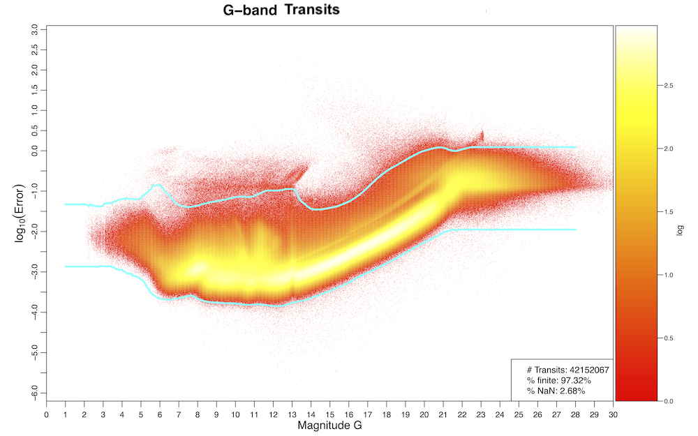
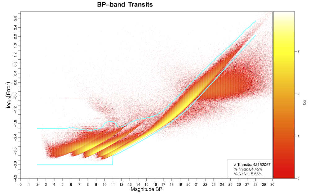
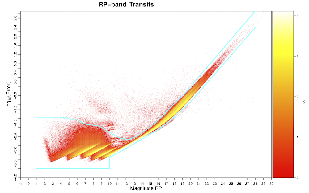
ExtremeErrorCleaningMagnitudeDependent: it was the last operator of the chain for the main processing in Gaia DR3. It removed individual transits above and below magnitude-dependent thresholds, which were determined as follows. From a sample of the photometric catalogue with at least 10 FoV transits in the band and for each band (limited to 6000 sources per 0.05 mag bin, for the golden, silver, and bronze data sets), we studied the quantile distribution of the transit magnitude errors and decided to use the 0.03 % and 99.7 % quantiles for the lower and upper limits, respectively, for data in the band. For both and , we used the 0.3 % and 99.9 % quantiles for the lower and upper limits, respectively. Figures 10.3–10.5 show the distributions of the transit magnitude errors as a function of the transit magnitudes, for the three Gaia bands, together with the thresholds used for this operator. The latter was not applied to per-CCD photometry.
-
8.
RemoveOutliersFaintAndBrightOperator: this operator was not used for the main processing steps (contrarily to Gaia DR2), but it was applied to specific work packages (e.g., eclipsing binaries, planetary transits, RR Lyrae stars, and Cepheids). It removed transits as follows (with configuration parameters described, where relevant, in the respective data product sections):
-
(a)
A measurement with an excessively large error (intrinsically or compared to some number of times the IQR of the uncertainties) is deemed an outlier and is removed.
-
(b)
Outliers at the extremes of the magnitude distribution of a time series are identified when their deviations from the median magnitude exceed a certain number of times the IQR (with different thresholds possible at the bright and faint ends). Such measurements are removed from the time series, unless they have similar outlying measurements in time or projected in magnitude.
-
(a)
-
9.
RemoveOutlierPerTransitOperator: it removed per-CCD outlier measurements per transit. This operator applied to per-CCD data only.
-
10.
ColorTimeSeriesOperator: it operated on two bands (like and ) and removed transits that were not in common with both bands, in order to return a colour time series.
The Gaia DR3 time series are published in the light_curve datalink table. The flag rejected_by_variability provides information on which transits in each band were rejected by the hierarchical chain of operators up to and including ExtremeErrorCleaningMagnitudeDependent. Downstream work packages might have rejected additional transits, e.g., by applying stricter thresholds for RemoveOutliersFaintAndBrightOperator, which however are not flagged in the Gaia DR3 archive. Other photometric flags (other_flags) were not used in variability processing.
For the processing of the radial velocity time series published in Gaia DR3, a simple operator (RvsOutlierRemovalOperator) removed NaN values and used a similar approach to that of RemoveOutliersFaintAndBrightOperator but using the median absolute deviation (MAD) instead of the IQR. Measurements beyond six times the MAD or 300, above or below the median of the radial velocity time series, were removed.
The SOS analysis of Long Period Variables further used the mean spectra. A simple operator (BpRpSpectraCut) cut measurements at both ends of the spectra by 7 array indices.
Published output
The Gaia DR3 photometric time series and variability flags, in addition to other information, are published in the light_curve datalink table. The radial velocity time series are published in the vari_epoch_radial_velocity table (Section 20.13.9).
Statistical parameter computation
Input
Clean photometric and radial velocity time series (Section 10.2.3) with at least one FoV transit.
Method
Following the pre-processing and basic time-series cleaning described in Section 10.2.3, the first step in the scientific processing chain is the computation of a number of descriptive, inferential, and correlation statistics for all time series. These parameters provide a first general overview of the data and their distributions and are used to determine whether variability is present in a time series of Gaia observations.
Descriptive statistics computed on the temporal evolution of the time series include (but are not limited to): the number of observations, time duration of the time series, mean of observation times,
Parameters that characterize the distribution of time series measurements and their uncertainties include the minimum, maximum, (trimmed) range, mean, median, standard deviation, skewness, kurtosis, point-to-point scatter (Abbe or von Neumann parameter; von Neumann 1941, 1942), interquartile range, median absolute deviation from the median, a measure related to the signal-to-noise ratio, and the highest ratio of absolute measurement deviations from the median to the measurement uncertainties.
Where applicable, sample-size unbiased weighted and unweighted estimators as well as robust estimates are computed and compared, as they can be useful in identifying outliers, transits assigned to the wrong sources or signatures of variability. Only unbiased unweighted and robust quantities are available for all Gaia DR3 time series in the Gaia catalogue.
The inferential test statistics used in Gaia DR3 included the Abbe hypothesis test (von Neumann 1941, 1942) as well as the and Stetson test statistics (Stetson 1996). These measures were used in the General Variability Detection (GVD, see Section 10.2.3), which classified time series as either variable or non-variable.
Stetson, Pearson, and Spearman correlation statistics are computed on all permutations of pairs of the three photometric bands (, , and ). The time series are filtered to remove unpaired observations and hence the correlations are computed on time series of equal length, containing only observations paired in the same transit.
Published output
Gaia DR3 statistical parameters of photometric time series are published in the vari_summary table and those of radial velocities in the vari_rad_vel_statistics table.
General variability detection
Input
As in the previous data releases, variability analyses were only performed on FoV averaged photometry in the , , and bands.
Method
The General Variability Detection (GVD) used a supervised classifier in order to identify potential variable sources. The training set contained 123 thousand sources from two classes:
-
•
almost 60 thousand variable sources from the selection of variables used in the training set of the general classification (described in Section 10.3);
-
•
about 63 thousand other objects (some of which might include low-amplitude variables, which however were not targeted for Gaia DR3), selected from the 75 % least variable sources in Gaia per magnitude interval.
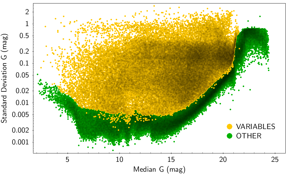
Figure 10.6 shows the standard deviation versus median magnitude of time series in the band, for the two training classes. An Extreme Gradient Boosting classifier (XGBoost; Chen and Guestrin 2016) was trained using time series statistics and other photometric quantities listed in the next paragraph. The estimated completeness was 99.3 % with a contamination of 0.37 % for the detection of variable sources. The trained classifier was applied to the photometric data set of Gaia with 5 FoV valid transits and the sources were classified as variable when the classifier posterior variability probability was larger than 50 %.
The classification attributes used to characterize variability included median_mag_g_fov, median_mag_rp, abbe_mag_g_fov, std_dev_mag_g_fov, qso_variability, range_mag_g_fov, the ratio std_dev_mag_bp over std_dev_mag_rp, the possibly reddened colour index median_mag_bp median_mag_rp, in addition to:
-
1.
a quantity distributed according to the null-hypothesis distribution of , given the data, for non-quasar objects, computed from a parameterized quasar variance model (Butler and Bloom 2011) after adaptation to the Gaia magnitudes of FoV transits in the band;
-
2.
the sample-size unbiased unweighted variance of FoV transit magnitudes in the band, denoised assuming Gaussian uncertainties (Rimoldini 2014);
-
3.
the difference between the of FoV transit magnitudes in the band and the mean of the distribution expected for constant objects (i.e., the number of degrees of freedom), normalised by the standard deviation of the distribution of constant objects (i.e., the square root of twice the number of degrees of freedom).
Published output
Period search and time series modelling
Input
Period search and Fourier modelling were applied to cleaned (Section 10.2.3) -band time series (expressed in magnitudes as a function of time in days) with 5 FoV transits, for sources identified as variable (Section 10.2.3). These methods rely also on the availability of statistical parameters (Section 10.2.3).
Method
The process of frequency (or period) search and time series modelling, collectively referred to as Variability Characterization, aims to characterize the variability behaviour of time series of Gaia measurements using a classical Fourier decomposition approach under the assumption that the light curve is mono- or multi-periodic. The goal is to produce, in an automated manner, the simplest and statistically most significant periodic model of the observed variability. For non-periodic light curves, this model is usually non-informative.
The general model fitted to Gaia time series for periodic variations in time is given by:
| (10.1) |
where is the degree of the polynomial model, is the number of detected frequencies, and is the maximum number of harmonics tested for frequency ; only the significant (not necessarily successive) harmonics are retained. The reference epoch is set to the middle of the time series and is already subtracted from the time .
Run-time configuration parameters
The configuration of the frequency search and model parameters is listed as follows:
-
1.
for frequency search:
-
(a)
at least five transits in the band,
-
(b)
no de-trending applied prior to the frequency search,
- (c)
-
(d)
minimum frequency of d (1429 d),
-
(e)
maximum frequency of 25 d ( min),
-
(f)
frequency step of d, where denotes the total time span of each time series,
-
(g)
refinement of the frequency about the most significant peak with a granularity of d;
-
(a)
-
2.
for modelling:
-
(a)
the polynomial model in Equation 10.1 was limited to degree zero, i.e., only the offset was fitted, without constant or higher order trends,
-
(b)
unweighted measurements were used in the fit,
-
(c)
non-linear fitting with the Levenberg-Marquard method was applied to the parameters of the final best model,
-
(d)
only one frequency was fitted, i.e., ,
-
(e)
with a maximum of up to 15 harmonics (only the significant ones are kept).
-
(a)
Published output
The output of period search was used as input for the general classification module (see Section 10.2.3). Some SOS work packages made use of both period search and modelling results.
General classification
The nTransits:5+ supervised classification aimed at classifying 25 different variability types, 24 of which are published among the variability tables (excluding galaxies). Figure 10.1 shows the list of published classes and the SOS work packages that depended on the classification results: AGN, Cepheid, compact companion, eclipsing binary, long-period variable, main-sequence oscillator, planetary transit, and RR Lyrae star. Further details of general classification are described in Section 10.3.
Published output
The nTransits:5+ classification results were published in the following Gaia DR3 tables: vari_classifier_definition, vari_classifier_class_definition, vari_classifier_result. Because of the artificial variability by which galaxies were identified, these classifications were removed from the variability tables and published in the galaxy_candidates table, where they can be found by setting the vari_best_class_name field equal to ‘GALAXY’.
Specific Object Studies
Objects of various classes of variables benefit from additional processing tailored to take into account specific properties of their variability. The Specific Object Study (SOS) components of the variability pipeline aim to characterize the time series and compute attributes specific to given variability types, which improve the identification and thus purity of their set of candidates. Each SOS module takes as input a list of candidates from one (or more) of the following inputs, as illustrated in Figure 10.1: (1) the relevant variability class(es) from the general classifier (Section 10.2.3), with probability thresholds specific to each SOS module, (2) a Special Variability Detection module (SVD), or (3) an extractor.
Details of the selection criteria, processing, and of the output data products of each SOS module are described in the respective data product sections.
Input
Source selections depend on specific SOS modules and are described in the relevant data product sections.
Method
Methods are described in the relevant data product sections.
Run-time configuration parameters
Run-time configuration parameters are described in the relevant data product sections.
Published output
An overview of all SOS related tables is provided in Section 10.1.2.