14.2 Internal comparisons 14.2.3 Photometry 14.2.5 Science Alerts

14.2.4 XP mean spectra

The construction of the XP mean spectra is described in Carrasco et al. (2021) and De Angeli et al. (2023). The latter also discusses the data quality and various issues detected.

Some general properties of the XP mean spectra in the catalogue can be found in Section 17.1.9 and Section 17.2.12.

In this section we describe some tests aiming for internal validation of the XP mean spectra in the catalogue. The tests look at some general properties (Section 14.2.4), the coefficients to the basis functions (Section 14.2.4), the shape of the spectra (Section 14.2.4), the integrated fluxes (Section 14.2.4), and the sampled spectra (Section 14.2.4).

General XP tests

Figure 14.9: Left: Histogram of the difference of the number of transits in BP with respect to RP used to build the mean spectra. Right: The same difference but using the number of observations used to build the mean photometry.

Empty spectra: There is (only) one source with an RP spectrum but no BP spectrum. This source is source_id $=5405570973190252288$ . It is a red and faint source ( $G=19.81$ , $G_{\rm BP}=21.76$ and $G_{\rm RP}=18.26$ mag). Although integrated photometry for BP could be calculated (using 11 observations), it is not surprising that no spectrum could be produced, given the faintness of the source.

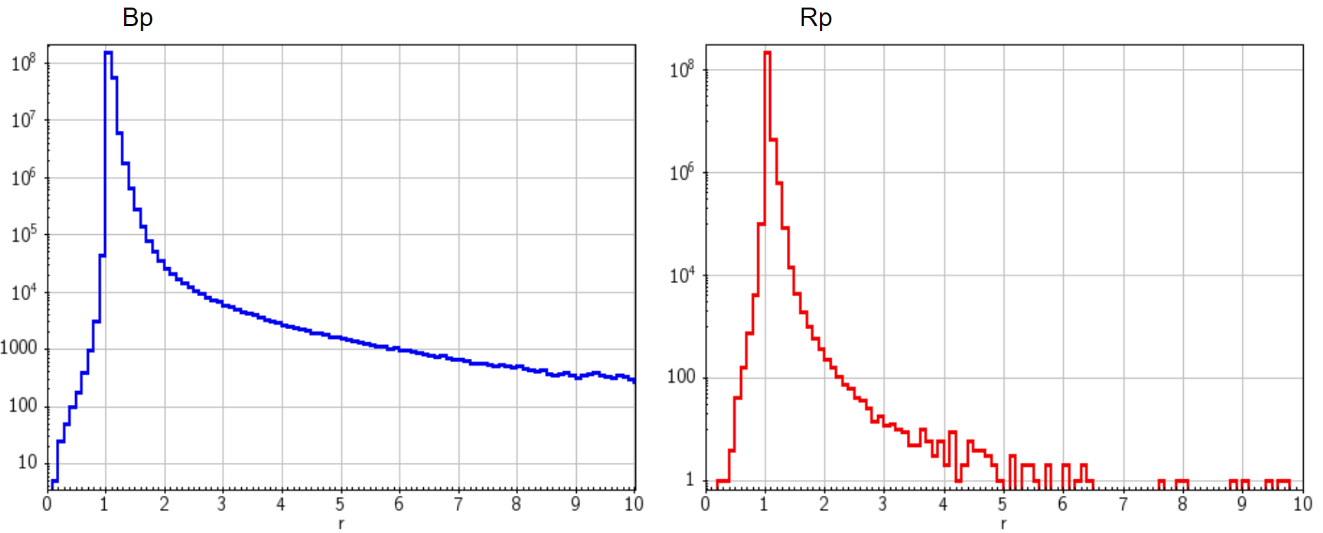
Number of transits: As can be seen in Figure 14.9, the number of transits used for building the mean BP spectra is lower than for the mean RP spectra, although the number of observations used to derive the mean photometry is more balanced. This is a known issue, resulting from the fact that BP spectra from the first ten months of mission were rejected due to contamination of the mirrors, cf. Section 1.3.3.

Tests on source coefficients

XP source coefficients absolute value: The absolute value of the XP source coefficients should be smaller (or of the same order of magnitude) than the integrated flux. If we define the XP (either BP or RP) mean spectra coefficients as $c^{\rm XP}_{i}$ and $F^{\rm phot}_{\rm XP}$ the XP flux derived from the photometric calibration (phot_bp_mean_flux or phot_rp_mean_flux), we flag sources with

|c^{\rm XP}_{i}|>k_{a}F^{\rm phot}_{\rm XP}\quad,

(14.1)

with being $k_{a}$ a proportionality factor, adopted here as $k_{a}=3$ . The index $i$ is running over all coefficients, i.e. $i=1,\ldots,55$ .

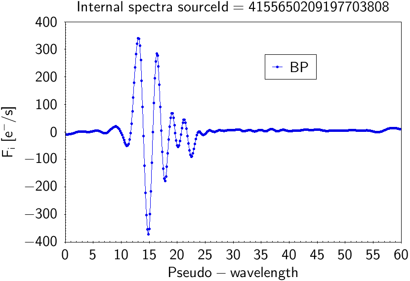
There is only one source failing the test for BP (none for RP), with source_id $=4155650209197703808$ . There are two coefficients of its BP spectrum not fulfilling $|c_{i}|<3F_{\rm BP}$ and failing the test. They are coefficients 33 and 37, having $c_{33}=-152.68$ and $c_{37}=-121.68$ respectively. This source is a blue and faint object ( $G=20.77$ mag, $G_{\rm BP}=21.33$ mag and $G_{\rm RP}=19.95$ mag). As it has very small total flux in BP ( $F_{\rm BP}^{\rm phot}=40.24\pm 23.16$ e ${}^{-}$ /s), its mean internal sampled BP spectrum is quite unrealistic (Figure 14.10). In fact, considering the error in the coefficients, they are compatible with zero.

Figure 14.10: Internal BP (blue) and RP (red) spectra for the source failing the test on the absolute value for the XP coefficients.

XP source coefficients decreasing: The values of the optimised XP source coefficients ( $c_{i}$ ) should in general be decreasing with the order of the coefficient ( $i$ ), see Figure 17.58. We consider the first $N_{limit}$ coefficients and test the difference

X=\sum\limits_{i=1}^{N_{limit}}|c_{i}|-\sum\limits_{i=N_{limit}+1}^{N_{coefs}}% |c_{i}|\quad.

(14.2)

Let $m$ be a vector of length $N_{coef}$ whose entries at position $i$ are $1$ if $c_{i}\geq 0$ and $-1$ else. We have to adjust the signs in the covariance matrix of the coefficients, $\Sigma^{c}$ , by computing $\Sigma^{c\prime}={\rm diag}(m)\,\Sigma^{c}\,{\rm diag}(m)$ . The error on $X$ is then given by

\sigma_{X}=\sqrt{\sum_{i,j=1}^{N_{limit}}\Sigma^{c\prime}_{i,i}+\sum_{i,j=N_{% limit+1}}^{N_{coef}}\Sigma^{c\prime}_{i,i}-2\cdot\sum_{i=1}^{N_{limit}}\sum_{j% ={N_{limit}+1}}^{N_{coef}}\Sigma^{c\prime}_{i,j}}\quad.

(14.3)

The test is passed for a source if

\frac{X}{\sigma_{X}}>-k\quad.

(14.4)

The suitable choice of the index $N_{\rm limit}$ depends on the basis in which the coefficients are analysed. For the optimised Hermite basis used in the spectra, a value of $N_{\rm limit}=5$ was adopted. For the limit, $k=5$ was used.

In Table 14.1 we show the results of the test.

Table 14.1: Testing that the source coefficients are decreasing.

Coefficients	% Passed	% Failed	Passed	Failed
BP	199.99%	0.01%	219 171 605	26 037
RP	100.00%	0.00%	219 192 173	15 470

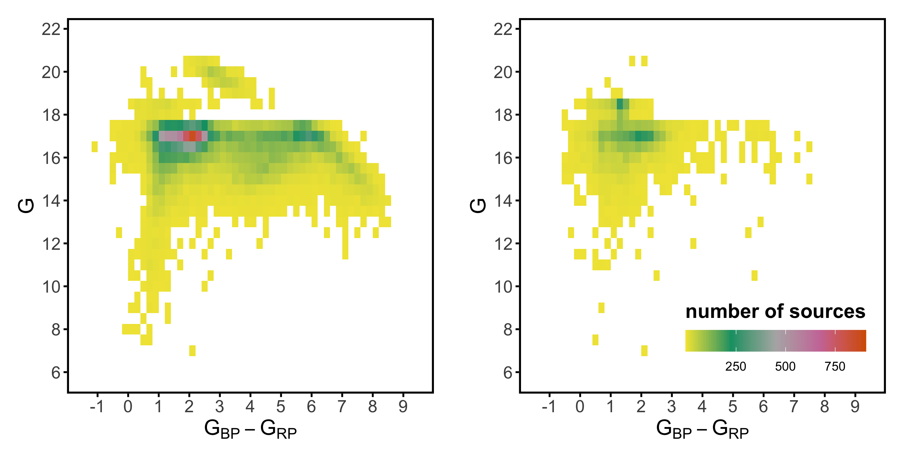
In Figure 14.11 we show the percentage of sources failing in a colour-magnitude diagram. Faint sources with extreme colours are the ones that fail the most, specially red sources for the BP test and vice versa.

Figure 14.11: Colour-Magnitude diagram of failing sources (in the optimised base) for decreasing coefficients test for BP (left) and RP (right).

Truncation of the number of coefficients: We check with this test that proposed truncation of the XP mean spectrum coefficients (according to bp_n_relevant_bases and rp_n_relevant_bases) produce good results.

We derive residuals as a function of the pseudo-wavelength of the sampled spectra derived using the full set of mean spectrum coefficients ( $f_{\lambda}^{\rm full}$ ) and the truncated set of coefficients ( $f_{\lambda}^{\rm trunc}$ ). We then compare this residual with the uncertainty in the sampled spectra using the full set of coefficients ( $\sigma_{f_{\lambda}^{\rm full}}$ ).

	$\displaystyle\text{mean}\left(\left\|\frac{f_{u}^{\rm full}(u_{i})-f_{u}^{\rm trunc% }(u_{i})}{\sigma_{f_{u}^{\rm full}}(u_{i})}\right\|\right)<k_{mn}$		(14.5)
	$\displaystyle\text{max}\left(\left\|\frac{f_{u}^{\rm full}(u_{i})-f_{u}^{\rm trunc% }(u_{i})}{\sigma_{f_{u}^{\rm full}}(u_{i})}\right\|\right)<k_{mx}$		(14.6)

with the values of $k_{mn}$ and $k_{mx}$ being the maximum number of standard deviations a spectrum in full representation and truncated representation is accepted to differ in mean and in maximum (we adopted $k_{mn}=1$ and $k_{mx}=3$ ).

In the wings, very large relative changes might be acceptable, as the count numbers are very small. The test is therefore done on two ranges of pseudo-wavelengths, one including the wings, and one without the wings. The sampling in the ranges for the two versions of the test is chosen as $u_{i}\in[0,60]$ and $u_{i}\in[15,45]$ in pseudo-wavelength space, using a sampling in 0.5 steps.

The test is passed for a source if it satisfies (14.5).

About $55$ – $60\%$ of the sources are considered failing this test when considering the whole XP spectrum and about $35$ – $40$ % when excluding the wings (see Table 14.2). The location of the failing sources in the sky show some correlation with the scanning law. The high numbers of failing sources is caused by the low threshold applied in this test. Comparing the failure rates with results from simulated data and the theoretical case of normally distributed data, the failure rate is about as expected.

Table 14.2: Results for coefficient truncation test for the two different intervals of pseudo-wavelength.

Band	% Passed	% Failed	Passed	Failed
$[0,60]$
BP	38.82%	61.18%	185 054 925	134 065 408
RP	45.84%	54.16%	100 440 777	118 679 557
$[15,45]$
BP	64.01%	35.99%	140 256 920	178 863 413
RP	60.46%	39.54%	132 473 460	186 646 874

Looking at the number of relevant basis functions for all the spectra, we find:

•

112 348 sources with bp_n_relevant_bases=1
•

0 sources with bp_n_relevant_bases=54
•

22 721 sources with bp_n_relevant_bases=55
•

75 430 sources with rp_n_relevant_bases=1
•

0 sources with rp_n_relevant_bases=54
•

5 sources with rp_n_relevant_bases=55

The first thing to notice is that there are no sources with relevant number of bases equal to 54. This is due a minor oversight and of little consequence. Another thing to notice is that there are very few sources (only 5) with relevant number of bases equal to 55 for RP. In fact, the spectra of sources with 55 relevant bases were checked to be pure noise and they have mostly $G_{\mathrm{BP}}-G_{\mathrm{RP}}>5$ mag. They have no significant coefficients and then the default value (55) is maintained.

Tests on the shape of the spectra

Beta angle: This test defines a set of representative sources located at different wide regions in the HR diagram and determines similarities in the XP spectrum for a given source with those in each of these regions. We use here the concept of ‘ $\beta$ angle’, which describes in a single parameter how well a spectrum can be represented as a linear combination of spectra in a set of reference spectra. This angle is thus always with respect to a certain set of reference spectra, and this set may change with application and purpose.

The test consists of selecting different sets of reference spectra, selected from different regions of the HR diagram. For all sources, the beta angle with respect to all selected reference were computed. Sources in the same region of the HR diagram as defined by a reference set should have small beta angles. Sources from different regions should have large beta angles. Non-stellar sources should have very large angles.

The integrated photometry and the parallax can be used to determine the position of sources in the HR diagram, and identify the reference sets for which the beta angle should be small. It is therefore necessary to apply the same selection criterion used for the selection of the reference sets to all test sources, and to classify them with respect to the reference sets.

Assume we have a set of $M$ XP spectra we use as the reference set. Each spectrum is represented by a vector ${\bf c}_{i}$ , $i=1,\ldots,N$ . To compensate for differences in brightness, we may normalise the spectra. A natural choice for the normalisation is the L2-norm. We denote the normalised vectors $\bar{\bf c}_{i}$ , with

\bar{\bf c}_{i}\coloneqq\frac{{\bf c}_{i}}{\sqrt{{\bf c}_{i}^{\mathsf{T}}\,{% \bf c}_{i}}}\quad,\quad i=1,\ldots,M\quad.

(14.7)

We then arrange the $M$ normalised vectors $\bar{\bf c}_{i}$ into the $M\times N$ matrix $\bf C$ and perform a Singular Value Decomposition on it, e.g.

{\bf C}={\bf U}\,{\boldsymbol{\Sigma}}\,{\bf V}^{\mathsf{T}}\quad.

(14.8)

We then use the $N\times N$ matrix $\bf V$ from this decomposition to construct a new basis for the XP spectra. Since this matrix is orthogonal by construction, i.e. ${\bf V}\,{\bf V}^{\mathsf{T}}=\mathbb{I}$ , we can multiply any spectrum $\bf c$ with ${\bf V}^{\mathsf{T}}$ , and if the sampled basis functions $\boldsymbol{\Phi}({\bf u})$ are multiplied with $\bf V$ , then the sampled spectra remain identical for any sampling $\bf u$ ,

\boldsymbol{\Phi}({\bf u})\,{\bf c}=\boldsymbol{\Phi}({\bf u})\,\mathbb{I}\,{% \bf c}=\boldsymbol{\Phi}({\bf u})\,{\bf V}\,{\bf V}^{\mathsf{T}}\,{\bf c}=% \left({\bf V}^{\mathsf{T}}\,\boldsymbol{\Phi}^{\mathsf{T}}({\bf u})\right)^{% \mathsf{T}}\,{\bf V}^{\mathsf{T}}\,{\bf c}\quad.

(14.9)

We are thus free to use an orthogonal matrix $\bf V$ to transform both the coefficients and the basis functions, without changing the representation of the spectra. The use of $\bf V$ from a SVD has the additional advantage that the new basis functions $\boldsymbol{\Phi}\,{\bf V}$ are sorted according to the singular values of the matrix $\bf C$ , ensuring that the basis functions are sorted according to their relevance in representing the set of $M$ reference spectra. We may therefore consider a truncation of the representation of the set of reference sources. We denote the number of transformed basis functions required to represent all spectra in the set of reference spectra to a satisfactory degree by $N^{\prime}$ , with $N^{\prime}<N$ . For the reference spectra we thus set coefficients for indices larger than $N^{\prime}$ to zero. For a source not within the set of reference spectra, its coefficients for indices larger than $N^{\prime}$ in comparison to all the coefficients provides a measure for how well the the spectrum can be represented by linear combinations of the spectra in the reference set.

We denote a coefficient vector in the transformed basis by ${\bf c}^{\prime}$ , i.e.

{\bf c}^{\prime}={\bf V}^{\mathsf{T}}\,{\bf c}\quad,

(14.10)

and the truncated vector resulting from setting all coefficients in ${\bf c}^{\prime}$ for indices larger than $N^{\prime}$ to zero we denote ${\bf c}^{\prime}_{tr}$ . The scalar product of ${\bf c}^{\prime}$ and ${\bf c}^{\prime}_{tr}$ can be expressed by the cosine of the angle between the two vectors, and we have

\cos\beta=\frac{{\bf c}^{\prime\,\mathsf{T}}_{tr}\,{\bf c}^{\prime}}{\sqrt{{% \bf c}^{\prime\,\mathsf{T}}_{tr}\,{\bf c}^{\prime}_{tr}\;{\bf c}^{\prime\,% \mathsf{T}}\,{\bf c}^{\prime}}}

(14.11)

This $\cos\beta$ is the quantity we are interested in. We may take the inverse cosine to obtain an angle directly. However, this is not strictly necessary and the non-linear transformation might have unfavourable effects in the computation of the error on $\beta$ for very noisy spectra. We therefore may prefer to use the cosine of $\beta$ instead of $\beta$ .

(14.11) simplifies further if we take into consideration that the first $N^{\prime}$ elements of ${\bf c}^{\prime}$ and ${\bf c}^{\prime}_{tr}$ are identical, and the remaining elements with indices $i=N^{\prime}+1,\ldots,N$ are identical zero. Therefore, ${\bf c}^{\prime\,\mathsf{T}}_{tr}\,{\bf c}^{\prime}={\bf c}^{\prime\,\mathsf{T% }}_{tr}\,{\bf c}^{\prime}_{tr}$ , and

\cos\beta=\sqrt{\frac{{\bf c}^{\prime\,\mathsf{T}}_{tr}\,{\bf c}^{\prime}_{tr}% }{{\bf c}^{\prime\,\mathsf{T}}\,{\bf c}^{\prime}}}\quad.

(14.12)

Graphically, this means the cosine beta is the ratio of the length of the coefficient vector containing only the coefficients required to describe the reference set of spectra, over the total length of the coefficient vector.

A suitable number of basis functions, $N^{\prime}$ , needs to be chosen for this test. To get this number, first, for all spectra in the reference set the value of $\beta$ can be computed as a function of the number of basis functions used, $n$ . Then, three different criteria may be applied to select $N^{\prime}$ :

•

The lowest $\beta$ in the set should be smaller than $l_{1}$ .
•

The highest $\beta$ in the set should be smaller than $l_{2}$ .
•

The median $\beta$ in the set should be smaller than $l_{3}$ .

The number $N^{\prime}$ of basis functions used is the smallest number that satisfies all three conditions together. The values chosen for the three thresholds are $l_{1}=1^{\circ}$ , $l_{2}=0.2^{\circ}$ , and $l_{3}=0.5^{\circ}$ .

We selected sources with good parallax (parallax_over_error $>5$ ) and computed the median $\beta$ angle of all sources within a cell in colour-magnitude grid with respect to several predefined populations.

The smaller the $\beta$ angle is, it means that a given source has a more similar spectrum with respect to those of the population.

We plot the distributions in the HR diagram in Figure 14.12 (BP) and Figure 14.13 (RP) for the populations: Main Sequence B (MSB), MSA, MSF, MSG, MSK, MSM, Red Clump and Subgiants.

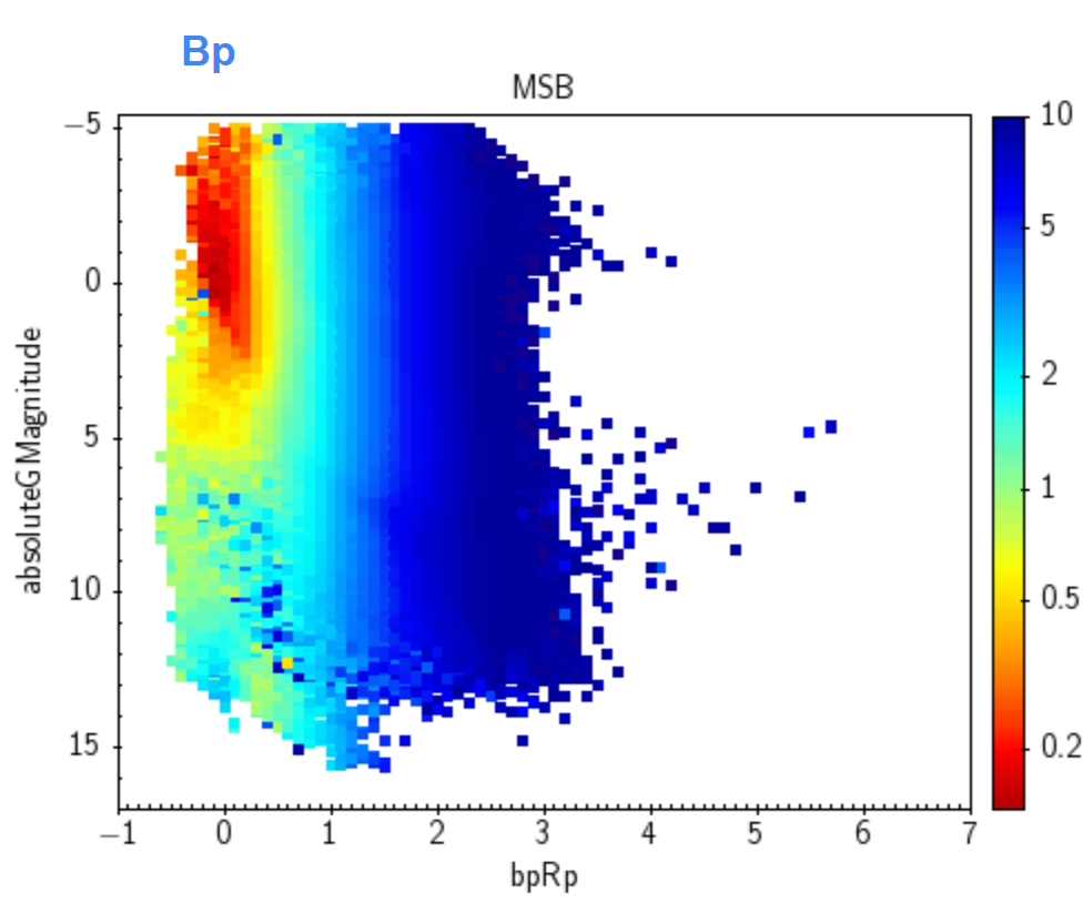
Figure 14.12: Beta angle in BP spectrum for Populations (from left to right, from top to bottom): Main Sequence B, A, F, G, K and M, Red Clump and Subgiants.

Figure 14.13: Same as in Figure 14.12 but for RP spectrum.

In general lines, all populations can more or less be distinguished from the others based on their XP spectra. Some populations are better detected in one of the bands. For example, MSK and MSM are clearly better detected in the RP spectrum, as only with the BP information one can only say that it is a red source, but not distinguish among different types of red source.

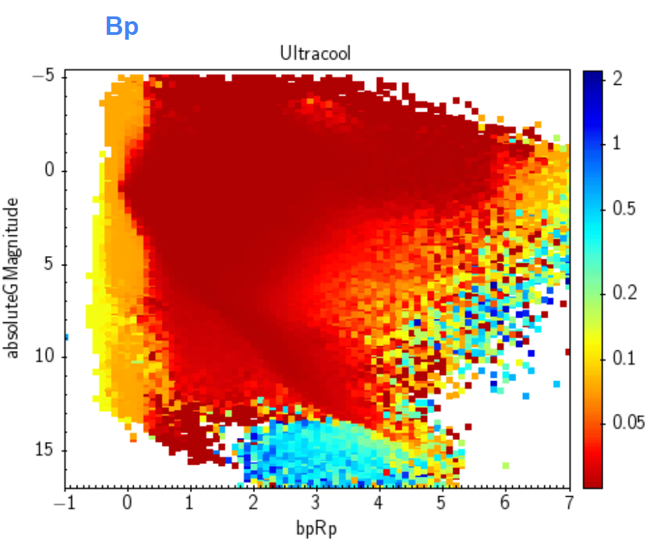
This feature is more exaggerated in the Ultra-cool case (Figure 14.14), which is completely non-discriminant in the BP case (with very low $\beta$ values as they are simply confused by faint sources at any colour interval) and improves considerably in the RP one, where low $\beta$ values are only present in the expected ultra-cool stars region. XP spectra alone cannot distinguish very well between main sequence and giants, as it can be seen with the vertical structures in the HR diagrams. Nevertheless, RP is more useful to distinguish Red Clump and subgiants.

Figure 14.14: Beta angle in BP (left) and RP (right) spectrum for the Ultra-cool population.

The same procedure was also carried out for White Dwarfs (WD). However, due to their faintness and the fact that they have a similar spectral shape with respect to other kinds of stellar sources, the $\beta$ angle is not enough to distinguish the subtle spectral differences to detect WDs correctly (Figure 14.15).

Figure 14.15: Beta angle in BP (left) and RP (right) spectrum for the White Dwarfs population.

Small wings: Values at the wings of the spectra should be smaller than in the central parts corresponding the wavelengths with significant response. To evaluate the behaviour of the spectra at the wings at both sides, we may consider the integrals over the spectra over finite intervals in pseudo-wavelength. We consider the expressions:

$\displaystyle I_{1}$	$\displaystyle\coloneqq$	$\displaystyle\int\limits_{-\infty}^{0}f(u)\,{\rm d}u$	(14.13)
$\displaystyle I_{2}$	$\displaystyle\coloneqq$	$\displaystyle\int\limits_{0}^{5}f(u)\,{\rm d}u$	(14.14)
$\displaystyle I_{3}$	$\displaystyle\coloneqq$	$\displaystyle\int\limits_{5}^{10}f(u)\,{\rm d}u\quad.$	(14.15)

And analogously on the other side of the spectrum:

$\displaystyle I_{4}$	$\displaystyle\coloneqq$	$\displaystyle\int\limits_{50}^{55}f(u)\,{\rm d}u$	(14.16)
$\displaystyle I_{5}$	$\displaystyle\coloneqq$	$\displaystyle\int\limits_{55}^{60}f(u)\,{\rm d}u$	(14.17)
$\displaystyle I_{6}$	$\displaystyle\coloneqq$	$\displaystyle\int\limits_{60}^{\infty}f(u)\,{\rm d}u\quad.$	(14.18)

One should find $I_{1}<I_{2}<I_{3}$ if the wings are decreasing. The integral $I_{1}$ tests the behaviour outside the range for which the basis functions have been constructed, and is sensitive to possible overshooting effects. The other side of the spectrum is in analogy, i.e. one should see $I_{4}>I_{5}>I_{6}$ , with $I_{6}$ testing the overshooting. We therefore consider the differences between pairs of these integrals, normalised to the uncertainty of the difference,

x_{ab}=\frac{I_{a}-I_{b}}{\sigma_{ab}}

(14.19)

with

\sigma_{ab}=\sqrt{\Sigma^{I}_{a,a}+\Sigma^{I}_{b,b}-2\Sigma^{I}_{a,b}}\quad.

(14.20)

Here, $\Sigma^{I}$ denotes the covariance matrix for the integrals. If we assume that the index $a$ refers to the outer interval, and $b$ to the inner one, then $I_{a}$ should in general be smaller than $I_{b}$ and we can chose a limit about what is acceptable for $x$ , say

x_{ab}<k

(14.21)

with the value $k=5$ adopted in the test.

This same test was repeated using truncated coefficients and the comparison is provided in Figure 14.16.

Figure 14.16: Comparison of the number of sources failing the small XP wings test when considering all source coefficients (solid lines) or only truncated ones (dotted lines) as a function of magnitude (left) and colour (right). BP in blue, RP in red.

The failing sources are not specially faint. In general the number of failing sources decrease when considering the truncated case. But it is surprising that for very red ( $G_{\mathrm{BP}}-G_{\mathrm{RP}}\sim 6$ mag) and bright ( $G<16$ mag) sources in RP the amount of failing sources increase when using truncated spectra.

Tests on integrated fluxes

Coherence between photometry and spectra: Integrated flux from XP spectra should be similar to the calibrated mean flux derived from the photometric calibration. See also Section 5.4.2.

Figure 14.17 shows the comparison of integrated photometry from XP spectra in the wavelength/pseudo-wavelength ranges [680 nm; 330 nm] = [14.223398; 51.402673] for BP and [680 nm; 1050 nm] = [11.228237; 48.919845] for RP (converted to magnitudes with the same zero points as in Gaia EDR3) and the mean photometry as a function of colour and magnitude. The samples for BP and RP contain about 1.0 and 1.7 million random sources brighter than $G_{\rm BP}=15$ mag and $G_{\rm RP}=15$ mag, respectively, and with good phot_bp_rp_excess_factor. Differences in zero points and dependencies with colour are expected (as shown in the top panels) because of the difference of the mean instruments in photometry and spectra. We notice, however, a dip in the RP comparison at about $G_{\rm RP}=9.5$ mag for the red sources ( $G_{\mathrm{BP}}-G_{\mathrm{RP}}>3.0$ ; bottom right panel), which is not explained.

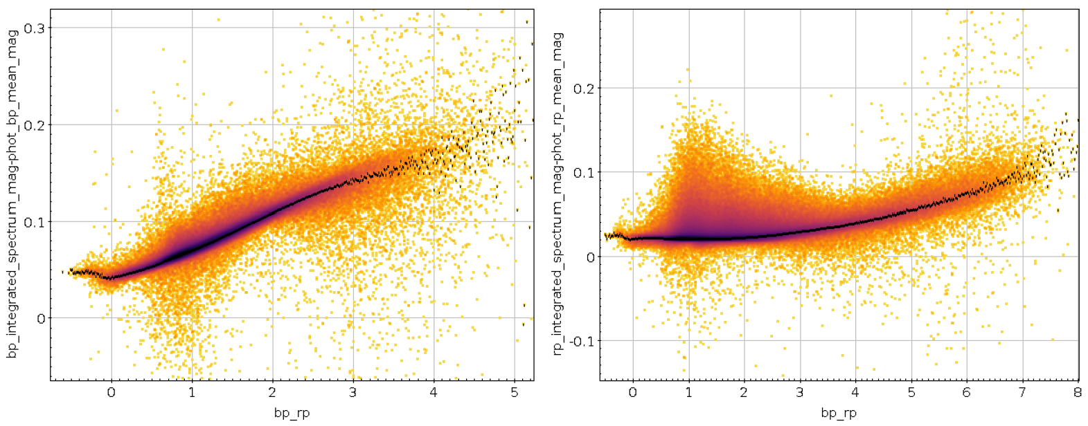
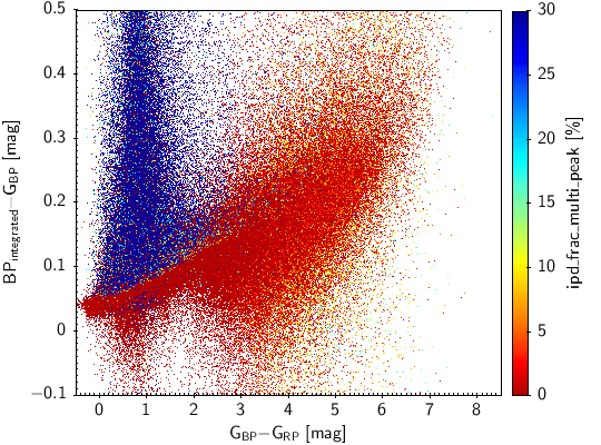
Figure 14.17: Top: Density graph of the differences between the integrated flux from XP spectra and the mean photometry in Gaia EDR3 as a function of the $G_{\mathrm{BP}}-G_{\mathrm{RP}}$ colour. Black points indicate the median of the differences. BP at the left plot; RP at the right plot. Bottom: Median of the differences as a function of magnitude. Different colours correspond to subsets of sources with different colour index.

The dip at $G_{\rm RP}=9.5$ mag in even deeper in Figure 14.18, where the same difference is shown but now versus the colour and for a larger sample ( $G_{\rm RP}<14$ mag). For $G_{\mathrm{BP}}-G_{\mathrm{RP}}$ between 4 and 5 mag the dip reaches 0.04 mag, but fading away for bluer colours and turning into an excess for very red sources. The plot also shows a population with excess for sources of normal colours. As shown in Figure 14.19, for the same sample, this is predominantly sources disturbed by another source closeby.

Figure 14.18: Difference between the integrated RP spectrum and the $G_{\rm RP}$ by colour for the 30.4 M sources brighter than $G_{\rm RP}$ = 14 mag. The median relation for different magnitude ranges is overplotted.

Figure 14.19: Difference between the integrated spectrum and the photometry by colour for BP and RP. The colour coding indicates the fraction of transits where the source showed an additional peak in the astrometric field.

In order to do this comparison for all sources in the catalogue with XP spectra, we define $F^{\rm phot}_{\rm XP}$ as the XP flux (either BP or RP) derived from the photometric passband calibration and $F^{\rm spec}_{\rm XP}$ the flux derived from the XP calibrated mean spectra. We now compute the ratio

r\coloneqq F^{\rm phot}_{\rm XP}/F^{\rm spec}_{\rm XP}

(14.22)

for all sources.

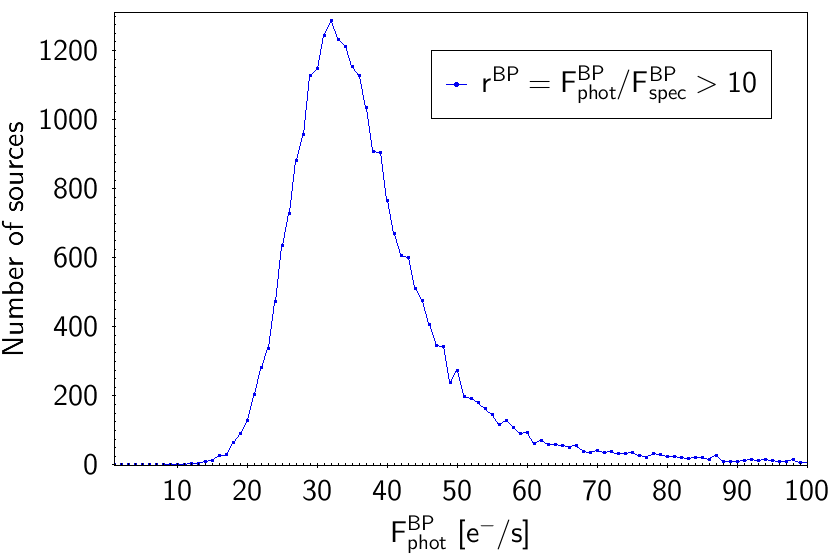
In Figure 14.20 we show the obtained $r$ distribution: both bands show a peak in $r=1$ , but in the BP case the tail to larger $r$ values (larger photometric flux than the spectral one) is wider than in the RP case.

Figure 14.20: Histogram of the ratio $r$ between the photometric and the spectrum flux in BP (left) and RP (right) for the integration of flux test.

The origin of this plateau at large $r$ values for BP could be related with the minimum values for BP fluxes (1 e ${}^{-}\mathrm{s}^{-1}$ ) imposed in Gaia DR3 photometry (see van Leeuwen 2021; Riello et al. 2021). When plotting the distribution of BP photometric fluxes for those sources having $r>10$ , (Figure 14.21) it can be seen that it peaks around $\langle F\rangle=32$ e ${}^{-}\mathrm{s}^{-1}$ instead. This correspond to the mean value expected when you cut half of the distribution when rejecting observations with fluxes smaller than 1 e ${}^{-}\mathrm{s}^{-1}$ ( $\langle F\rangle\sim\sqrt{\frac{2}{\pi}}\cdot\sigma$ , obtaining $\sigma\sim 40$ e ${}^{-}\mathrm{s}^{-1}$ ).

Figure 14.21: Histogram of the flux in BP for those sources having $r^{\rm BP}=F_{\rm phot}^{\rm BP}/F_{\rm spec}^{\rm BP}>10$ .

Uncertainty of the integrated flux: In this test the integrated flux uncertainty from XP spectra is compared with the uncertainty in the flux derived from the integrated passband calibration.

For this end, we compare the uncertainty in the integrated flux derived from the photometric calibration ( $\sigma_{F^{\rm phot}_{\rm XP}}$ ) with the uncertainty in the integrated flux derived from the spectra ( $\sigma_{F^{\rm spec}_{\rm XP}}$ ).

\kappa\coloneqq\frac{\sigma_{F^{\rm phot}_{\rm XP}}}{\sigma_{F^{\rm spec}_{\rm XP% }}}

(14.23)

In Figure 14.22 we show the obtained distribution showing a peak near $\log_{10}(k)=0$ , although a bit deviated to positive $k$ values (larger photometric uncertainties). Besides, the widths of the distributions are a bit wide. Taking into account that we plot the logarithm of $k$ , we find excessive to have a ratio between the two flux errors of a factor $10^{3}-10^{4}$ larger or smaller.

Figure 14.22: Histogram of the ratio $k$ between the photometric and the spectrum flux error in BP (left) and RP (right) for the error in the integration of flux test.

Negative integrated fluxes in the spectra: Spectra should not have negative fluxes, with the exception of noise for sufficiently faint sources.

We may quantify the degree of ‘negativity’ of a spectrum be the quantity

z=\frac{\int\limits_{-\infty}^{\infty}\left|f(u)\right|\,{\rm d}u-\int\limits_% {-\infty}^{\infty}f(u)\,{\rm d}u}{2\,\int\limits_{-\infty}^{\infty}\left|f(u)% \right|\,{\rm d}u}\quad.

(14.24)

Here,

\int\limits_{-\infty}^{\infty}\left|f(u)\right|\,{\rm d}u\equiv||f(u)||_{1}

(14.25)

is the $l1$ –norm of the spectrum. If there are no negative fluxes within the spectrum, this value should be zero. If there are only negative values, it gives one. The more negative values there are in a spectrum, the larger this number $z$ should get.

Unusual values of $z$ can be identified by looking at a plot of $z$ against the $l1$ –norm. The sources with very high values of $z$ may be affected by an over-subtraction of the sky background. We expect the negativity to follow a logarithmic relation with the norm of the spectrum $||f(u)||_{1}$ . We approximated this relation by $0.02+10^{-1.2(||f(u)||-2)}$ and marked as failed any spectrum above this function. Moreover, any spectrum with more than 90% of negativity is also flagged.

Only 2438 and 550 sources are failing this test, in BP and RP respectively. Figure 14.23 shows the distribution of the spectra in a negativity-flux diagram.

Figure 14.23: Negativity vs. flux norm diagram in BP (left) and RP (right) for the negative integrated flux test.

Excess flux: This test compares excess flux from the spectra with excess flux from the photometry. The criterion for a failing source is that $|e^{\rm phot}-e^{\rm spec}|>5$ , being $e^{\rm phot}$ and $e^{\rm spec}$ the photometric and spectrophotometric excess fluxes, respectively. Only 82 sources are failing this test, being mostly the faintest sources in the sample.

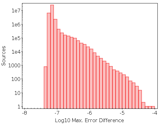
Mean sampled spectra

This test checks that the mean sampled spectra dataset is correctly built from the source coefficients with differences compatible with floating point accuracy. If there is an error in the computation, then it should show in basically all sources. We derive an independent set of sampled spectra and compute their relative difference with respect to the published (sampled) spectra. The maximum absolute value of this relative difference for a source is the quantity of interest. Figure 14.24 shows that value of the discrepancy is very small, concluding that the mean spectra have been correctly built from the coefficients.

gaia data release 3 documentation