1.1 The Gaia mission
1.1.1 Introduction and overview
Author(s): Jos de Bruijne
This is the online documentation of Gaia Data Release 1 (Gaia DR1; click here for the full pdf version). This documentation has been prepared as background information to the Gaia papers in the Special Issue of A&A that accompanies Gaia DR1. Gaia Collaboration et al. (2016b) describes the Gaia mission. Gaia Collaboration et al. (2016a) provides an overview of the contents of Gaia DR1. Arenou et al. (2017) describes the overall validation of the data. The data itself is available from the Gaia Archive at http://archives.esac.esa.int/gaia. The Gaia mission home page is https://www.cosmos.esa.int/gaia/.
1.1.2 Mission history and science case
Author(s): Jos de Bruijne
Hipparcos legacy
Whereas astrometry originated several millennia ago (for an overview, see Perryman 2012), the last centuries – and the last decades in particular – have shown exponential progress in the number of objects and the accuracy with which their positions, proper motions, and parallaxes are determined. These improvements have arisen as a result of improved technologies and instrumentation and of the possibility to eliminate the effects of the Earth’s atmosphere by going to space. Astrometry from space was pioneered by ESA’s Hipparcos mission, which operated from 1989 till 1993. The Hipparcos Catalogue was published in 1997 (ESA 1997; van Leeuwen 2007). An overview of the science revolution that Hipparcos has brought about is presented by Perryman (2009).
Hipparcos’ successor, originally named GAIA, was proposed in the early 1990’s by Perryman and Lindegren as an interferometric concept (Lindegren and Perryman 1995). Later, the mission design was changed to a direct-imaging approach but the name was kept for continuity reasons yet spelt as of then with small letters, i.e., Gaia. For more details about the history of Gaia, see Høg (2011, 2014).
Objectives of Gaia
The main science goal of Gaia is to unravel the structure, dynamics, and chemo-dynamical evolution of the Milky Way through the observation of one billion constituent stars. The data comprises astrometry and low-resolution spectro-photometry. For the brightest subset of targets, spectra are acquired to obtain radial velocities. The full list of Gaia’s science objectives is defined in Perryman et al. (2001) and summarised in Gaia Collaboration et al. (2016b).
1.1.3 The spacecraft
Author(s): Jos de Bruijne, Juanma Fleitas, Alcione Mora
Overview
The spacecraft consists of a payload module with the instrument and a service module with support functions. The prime contractor of Gaia is Airbus Defence and Space, Toulouse, France (formerly known as Astrium). An overview of the spacecraft is provided in Gaia Collaboration et al. (2016b).
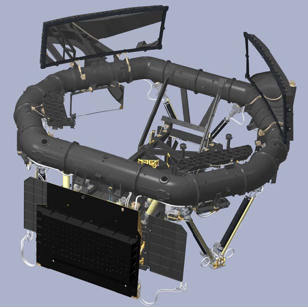
Payload Module
The payload module houses the two telescopes and the focal plane. In addition, the payload houses the focal-plane computers (the video-processing units, running the video-processing algorithms), the detector electronics (PEM), an atomic master clock, metrology systems (basic-angle monitor and wave-front sensors), and the payload data-handling unit. An overview of the payload module can be found in de Bruijne et al. (2010); Gaia Collaboration et al. (2016b).
Telescopes
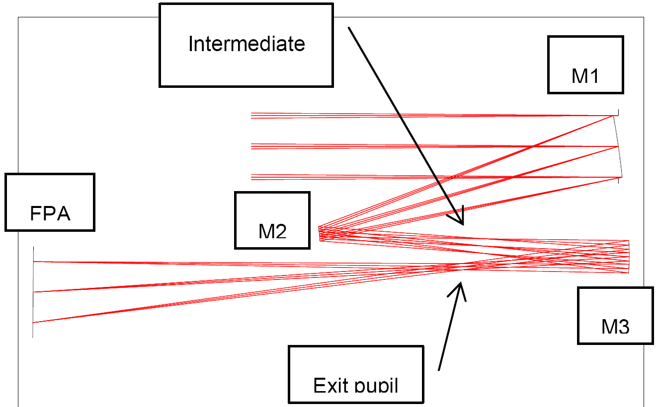
Gaia houses two telescopes, sharing a common focal plane. The lines of sight of the telescopes are separated by the basic angle. Both telescopes are three-mirror anastigmats with a Korsch off-axis configuration. The input pupils are located at the rectangular primary mirrors, and have a dimension of 1.450.5 m. A beam combiner at the exit pupil merges the optical paths. Two further flat mirrors in the combined beam fold the light towards the focal plane. The total number of mirrors is hence 10. An overview of the optical layout is displayed in Figure 1.1. More details on the telescopes are given in Gaia Collaboration et al. (2016b).
 |
 |
The focal length of both telescopes is 35 m, providing a plate scale of 58.9 176.8 mas pixel in the along- and across-scan directions, respectively. The rectangular aperture allows one-dimensional binning of CCD images in the across-scan direction for faint stars, substantially reducing the CCD readout noise and down-link bandwith, with minimum impact on the astrometry.
The focal plane
The focal plane is shared by both telescopes. It houses 106 charge-coupled-device (CCD) detectors. Since Gaia is continuously scanning around its axis, the CCDs are operated in time-delayed integration (TDI) mode. Gaia’s measurements are very precise in the scan direction through precise timing of the signals (line-spread functions, LSFs). The focal plane houses five functionalities:
-
•
metrology: a basic-angle monitor composed of two detectors (one nominal and one redundant) continuously measures variations in the basic angle between the two telescopes. Two wave-front sensors allow monitoring the optical quality of the telescopes;
-
•
sky mapping: both telescopes have their own sky-mapper (SM) detectors (14 devices in total). These detectors allow detecting objects of interest (point sources as well as slightly extended sources such as asteroids and unresolved galaxies) and rejecting cosmic rays, Solar protons, etc.;
-
•
astrometry: 62 CCDs are devoted to astrometry in the so-called astrometric field (AF);
-
•
spectro-photometry: 14 CCDs are devoted to low-resolution spectro-photometry. Spectra, dispersed along the scan direction, are generated through the use of a blue and a red prism (blue and red photometers, BP and RP);
-
•
spectroscopy: 12 CCDs are devoted to spectroscopy. Medium-resolution spectra (, dispersed along the scan direction) are generated through an integral-field grating plate.
More details on the focal plane can be found in Gaia Collaboration et al. (2016b).
Video Processing Unit and Algorithms
The CCDs in the focal plane are commanded by video-processing units (VPUs). Gaia has seven identical VPUs, each one dealing with a dedicated row of CCDs. Each CCD row, contains in order, two SM CCDs (one for each telescope), 9 AF CCDs, 1 BP CCD, 1 RP CCD, and 3 RVS CCDs (the latter only for four of the seven CCD rows). The VPUs run seven identical instances of the video-processing algorithms (VPAs), not necessarily with exactly the same parameter settings though. This (mix of some hardware and mostly) software is responsible for object detection (after local background subtraction), object windowing (see below), window conflict resolution, data binning, data prioritisation, science-packet generation, data compression, etc. More details can be found in Gaia Collaboration et al. (2016b).
The Sky Mapper (SM) CCDs are systematically read in full-frame mode. The object-detection chains for SM1 and SM2 are functionally identical, but their processing algorithms are parametrised independently. The detection algorithms scan the images coming from each SM in search for local flux maxima. A basic data treatment is applied correcting from gain and offset per sample. For each detected local maximum, spatial-frequency filters in both the along- and the across-scan directions are applied to the flux distribution within a samples working window centred on the local maximum. Objects failing to meet star-like PSF criteria are classified as prompt-particle-event (PPE) or (bright-star) ripple, high-frequency or low-frequency outliers, respectively.
The surviving detections are classified either as faint detected object or saturated extremity. They are sorted by flux and subsequently up to a maximum of 5 objects per TDI line per field-of-view are retained in view of memory sizing constraints. A list of detected objects is then produced with their attributes, mainly magnitude computed from the flux collected, observation priority, class of sampling, type, and along- and across-scan position. Saturated extremities are combined together to produce bright-star detections. Finally, Virtual Objects (VOs) are ‘artificially’ added to the list of detected objects.
After that, the available resources for observation in the AF instrument are allocated to the list of SM-detected objects according to their priority (essentially magnitude). Some SM-detected objects may be discarded at this stage due to a lack of resources; this is especially true during Galactic-plane scans (GPSs). Finally, a filtering stage using AF1 data either confirms the objects for observation or discards them if no corresponding signal is observed in AF1. Only the confirmed objects with AF1 data are observed in the whole AF instrument (AF2–AF9). The observation windows, which are assigned according to the object’s sampling class, are centred on the object and have an initial rectangular shape. Across-scan sample propagation in each field-of-view and conflict management among windows from different objects and CCD boundaries, possibly resulting in sample truncation, determine the final window shape and sample size per object.
As the objects reach the end of the AF instrument, similar algorithms as the ones described for AF are triggered for BP/RP. A new resource-allocation process is carried out, for BP and RP independently, optimising the observations based on the object priority while ensuring a constant number of samples per TDI line. The observation windows which are assigned according to the class of sampling of the object, are centred on the object and shaped by the field-of-view-dependent across-scan propagation, window conflicts, and CCD boundaries.
After the SM, AF, and BP/RP raw samples have been observed for an object, they are grouped to form a star packet of type 1 (SP1) and stored in the payload data-handling unit (PDHU; Section 1.1.3). When gathering the raw samples, the VPU limits the exposure time for bright stars by activating the user-defined TDI gate, both in the AF and in the BP/RP CCDs. However, SM CCDs are operated with Gate 12 permanently active to avoid excessive saturation from bright stars. Finally, in order to minimise the effect of CTI due to charge trapping, a periodic charge injection (CI) is activated in each AF and BP/RP CCD. The shape of the windows is recorded in the SP1 packet header in order to facilitate the window-reconstruction process on-ground. Each SP1 packet is time stamped with the object acquisition time in AF1. The packet is assigned a File_ID for PDHU storage and down-link prioritisation.
With part of the flux collected from the RP spectrum, an estimation of the magnitude of the object in the RVS instrument is produced. When this is not possible, the RVS magnitude is computed as an extrapolation from the AF magnitude. The object observation priority and class of sampling in RVS is derived from this magnitude. A separate resource-allocation process is carried out for the RVS. The observation windows, which are assigned according to the class of sampling of the object, are centred on the object and are shaped by the field-of-view-dependent across-scan propagation, conflict management, and CCD boundaries.
After the RVS raw samples have been collected for an object, they are grouped to form a star packet of type 2 (SP2) and stored in the PDHU. In RVS CCDs charge injections and gates are not applied. The shape of the windows is recorded in the header of the SP2 packet. Each SP2 packet is time stamped with the object acquisition time in AF1 and the packet is assigned a File_ID for PDHU storage and down-link prioritisation.
Payload Data-Handling Unit
Science packets generated on board are stored in the payload data-handling unit (PDHU) before being down-linked to ground. Under normal sky conditions, the PDHU can contain several days worth of science data. When the scanning law makes Gaia scan (roughly) along the Galactic plane for several consecutive days, however, the PDHU saturates and a user-defined prioritisation scheme comes in play to govern data deletion. More details on the PDHU are provided in Gaia Collaboration et al. (2016b).
Clock Distribution Unit
The clocking of all CCD detectors is based on a high-accuracy atomic clock, embedded in the clock distribution unit (CDU). More details on the CDU are contained in Gaia Collaboration et al. (2016b).
Wave-Front Sensor
Two CCDs in the focal plane are equipped with wave-front sensors (WFSs) to enable monitoring the optical quality of the telescopes. See Gaia Collaboration et al. (2016b) for details.
Basic-Angle Monitor
Two CCDs in the focal plane are part of the basic-angle monitor (BAM). The BAM allows monitoring variations of the basic angle of the telescopes to as-levels every 15 minutes. More details are provided in Gaia Collaboration et al. (2016b).
Astrometric instrument
The astrometric field (AF) contains 9 CCD strips and 7 CCD rows (it contains 62 CCDs since one CCD is sacrificed for the WFS). The bandpass of the AF detectors, defining the Gaia band, covers 330–1050 nm; this is mainly set by the telescope transmission in the blue and the CCD response in the red. The AF CCDs are not read out in full but only ‘windows’ around objects of interest are read out. The typical window for faint stars is pixels (along-scan across-scan), with the 12 pixels in the across-scan direction typically binned on chip into one single number (the intensity of the along-scan LSF). For bright stars, single-pixel-resolution windows are used, of size pixels (along-scan across-scan). For more details on the astrometric instrument, see Gaia Collaboration et al. (2016b).
Photometric instrument
The photometric instrument contains 2 CCD strips and 7 CCD rows. Half of the CCDs are devoted to the blue photometer (BP, covering 330–680 nm) and the other half are devoted to the red photometer (RP, covering 640–1050 nm). Dispersion of light takes places in the along-scan direction and windows measure pixels (along-scan across-scan). For more details on the astrometric instrument, see Gaia Collaboration et al. (2016b).
Spectroscopic instrument
The spectroscopic instrument contains 3 CCD strips and 4 CCD rows. Dispersion of light takes places in the along-scan direction and windows measure pixels (along-scan across-scan). For more details on the spectroscopic instrument, see Gaia Collaboration et al. (2016b).
Service Module
The service module (SVM) supports the payload, both mechanically / structurally and electronically / functionally. A description of the service module can be found in Gaia Collaboration et al. (2016b).
1.1.4 The scanning law
Author(s): Jos de Bruijne
The scanning law of Gaia determines how Gaia scans the sky. It is explained in Gaia Collaboration et al. (2016b). The scanning motion consists of two, effectively independent components: a six-hour rotation around the spin axis, and a 63-day precession (at fixed Solar-aspect angle) of the spin axis around the Solar direction. This enables full-sky coverage every few months and, on average, 70 focal-plane transits over the nominal, five-year mission.
Ecliptic-Pole Scanning Law
Nominal Scanning Law
1.1.5 Ground segment and operations
Author(s): Jos de Bruijne
Mission operations
Mission operations are conducted from the ESA Mission Operations Centre (MOC), located at the European Space Operations Centre (ESOC), Darmstadt, Germany. Mission operations include mission planning, regular upload of the planning products to the mission time line of Gaia, acquisition and distribution of science telemetry, acquisition, monitoring and analysis, and distribution of health, performance (voltage, current, temperature, etc.), and resource (power, propellant, link budget, etc.) housekeeping data of all spacecraft units, performing and monitoring operational time synchronisation, anomaly investigation, mitigation, and recovery, orbit prediction, reconstruction, monitoring, and control, spacecraft calibrations (e.g., star-tracker alignment, micro-propulsion offset calibration, etc.), and on-board software maintenance. Details are provided in Gaia Collaboration et al. (2016b).
Science operations
Science operations are conducted from the ESA Science Operations Centre (SOC), located at the European Space Astronomy Centre (ESAC), Madrid, Spain. Science operations include generating the scanning law, including the associated calibration of the representation of the azimuth of the Sun in the scanning reference system in the VPU software (Section 1.3.3), generating the science schedule, i.e., the predicted on-board data rate according to the operational scanning law and a sky model, to allow for adaptive ground-station scheduling, generating the avoidance file containing time periods when interruptions to science collection would prove particularly detrimental to the final mission products, generating payload operation requests, i.e., VPU-parameter updates (e.g., TDI-gating scheme or CCD-defect updates), tracking the status and history of payload-configuration parameters in the configuration database (CDB) through the mission time line and tele command history, hosting the science-telemetry archive, generating event anomaly reports (EARs) to inform downstream processing systems of ‘bad time intervals’, outages in the science data, or any (on-board) events which may have an impact on the data processing and/or calibration, monitoring (and recalibrating as needed) the star-packet-compression performance, monitoring (and recalibrating as needed) the BAM laser-beam-waist location inside the readout windows, reformatting the optical observations of Gaia received from Gaia’s Ground-Based Optical Tracking (GBOT) programme for processing in the orbit reconstruction at the MOC, and disseminating meteorological ground-station data – required for delay corrections in the high-accuracy time synchronisation – from MOC to DPAC. Details are provided in Gaia Collaboration et al. (2016b).
Bright-star handling
Stars brighter than 3 mag in the Gaia band are not properly detected on-board on each transit. Special, so-called SIF data are therefore acquired for them in the sky-mapper (SM) CCDs. See Gaia Collaboration et al. (2016b) for details.
Dense-area handling
Gaia cannot cope with infinitely dense areas on the sky. As explained in Gaia Collaboration et al. (2016b), the crowding limit is a few objects per square degree for astrometry and photometry; for spectroscopy, the limit is around objects per square degree. For a handful of selected, dense areas (e.g., Baade’s Window and Cen), special SIF data are acquired in the sky-mapper CCDs to support the deblending of data in the ground processing. More details are provided in Gaia Collaboration et al. (2016b).