3.4 Processing steps

Author(s): Jose Hernandez

The AGIS pre-processing takes care of preparing the data produced by other systems which is needed by AGIS to arrange and convert the data in a way which will be more suited for the AGIS execution.

The types of data used by AGIS are:

• •

  The Gaia satellite and main solar-system bodies ephemeris.

• •

  The time ephemeris needed to convert between the different time scales used in DPAC processing (OBMT, TCB, etc.).

• •

  The current Gaia DPAC source catalogue originating from the IGSL.

• •

  The IDT or IDU AstroElementaries (FOV Observations, each one typically containing 1 SM CCD transit and 8 or 9 AF CCD transits), in the first release only IDT AstroElementaries were used.

• •

  The IDU match information, linking AstroElementaries with Gaia catalogue sources.

• •

  The IDU new sources which were created during the AstroElementary to Gaia catalogue match process.

• •

  The commanded attitude files, used to generate the initial attitude needed to bootstrap AGIS.

• •

  The BAM data was analysed offline in order to find out the discontinuities where calibration boundaries should be placed.

AGIS works internally in the TCB time scale while typically most of the input data coming from the MDB are tagged in OBMT, during the pre-processing the OBMT times get converted into TCB times.

The pre-processing also takes care of filtering those CCD transits where the IPD was not successful as reported in the corresponding IDT/IDU flags provided in the AstroElementary, during the pre-processing the sources and their observations are sorted so that during the AGIS processing all the observations of each source are available to the core algorithm computing the source parameters.

At the end of the pre-processing we have the source catalogue and the observations arranged in a convenient way for the AGIS processing. The next step consists of the selection of the primary sources and their associated Gaia observations. These are the sources which will be used in the iterative process to determine the nuisance parameters (Attitude and Calibration). In DR1 the primary selection was done in a special way as the set consisted of the Hipparcos and Tycho-2 sources with their priors (see Section 4.2.3) (so a special module (TgasDataSelector) was executed in order to find and extract from the whole input data the Hipparcos and Tycho-2 sources, read in the original catalogues and populate the prior information. The TgasDataSelector task also selected only those sources which had a minimum of three telescope transits (AstroElementaries), as a result 2 482 282 sources where selected as primaries: 120 385 from the HIP2 catalogue and 2 361 897 sources from the Tycho-22 catalogue.

Author(s): Uwe Lammers

The Gaia core solution aims to solve the astrometric parameters for more than 1 billion sources mainly in our Galaxy. This clearly presents an enormous computational challenge as the size of the data set, and the large number of parameters, cannot be processed sequentially. The difficulty is caused by the strong connectivity among the observations: each source is effectively observed relative to a large number of other sources simultaneously in the field of view, or in the complementary field of view some ${106.5}^{\circ }$ away on the sky, linked together by the attitude and calibration models. The complexity of the astrometric solution in terms of the connectivity between the sources provided by the attitude modelling was analysed by Bombrun et al. (2010), who concluded that a direct solution is infeasible, by many orders of magnitude, with today’s computational capabilities. The study neglected the additional connectivity due to the calibration model, which makes the problem even more unrealistic to attack by a direct method. Note that this is not a defect, but a virtue of the mathematical system under consideration: it guarantees that a unique, coherent and completely independent global solution for the whole sky can be derived from the system.

To overcome this difficulty an iterative method has been developed over a number of years using increasingly complex and efficient algorithms. This approach became known as the Astrometric Global Iterative Solution (AGIS) and now relies on a Conjugate Gradient (CG) algorithm to converge the solution efficiently (Bombrun et al. 2012). The numerical approach to AGIS is a block-iterative least-squares solution. In its simplest form, four blocks are evaluated in a cyclic sequence until convergence. The blocks map to the four different kinds of unknowns outlined in Section 3.1.1, namely:

• S:

  the source (star) update, in which the astrometric parameters $𝒔$ of the primary sources are improved;

• A:

  the attitude update, in which the attitude parameters $𝒂$ are improved;

• C:

  the calibration update, in which the calibration parameters $𝒄$ are improved;

• G:

  the global update, in which the global parameters $𝒈$ are improved.

The G block is optional, and will perhaps only be used in some of the final solutions, since the global parameters can normally be assumed to be known a priori to high accuracy. The blocks must be iterated because each one of them needs data from the three other processes. For example, when computing the astrometric parameters in the S block, the attitude, calibration and global parameters are taken from the previous iteration. The resulting (updated) astrometric parameters are used the next time the A block is run, and so on. The mathematical description of the AGIS block-iterative least-squares solution and the updating of each block has been outlined in detail in Sections 4 and 5 respectively of Lindegren et al. (2012). In addition to these blocks, separate processes are required for the alignment of the astrometric solution with the ICRS (see also Section 3.3.2), the selection of primary sources, and the calculation of standard uncertainties; these auxiliary processes are discussed in (Section 6 of Lindegren et al. 2012).

Additionally, it is not necessary for the AGIS solution to include all one billion sources. Instead, it is done using a selection of about 10% of the astrometrically well behaved single sources and this is sufficient to converge the attitude and calibration solutions. The other sources can then be solved for in a secondary solution (see Section 3.4.3) using the converged parameters found in the primary AGIS solution. The primary solution will consist of about ${10}^8$ sources so the number of unknowns in the global minimization problem is about $5\times {10}^8$ for the sources ($𝒔$), $4\times {10}^7$ for the attitude ($𝒂$, assuming a knot interval of 15 s for the 5 yr mission; ${10}^6$ for the calibration $𝒄$, and less than 100 global parameters ($𝒈$). The number of elementary observations ($l$) considered is about $8\times {10}^{10}$.

Author(s): Jose Hernandez

The converged attitude and calibration obtained in the primary solution were used to do a source update on all the sources which had at least one AstroElementary with valid AF transits matched to them. This process is called the secondary source processing. 2,578,806,414 sources where treated and a solution was obtained for 1,466,675,582 of them. The attitude used was in the DR1 reference frame which automatically ensures that all the source positions for the secondary set are also in the same reference frame.

The solution was done performing a 5-parameter update using priors for the parallax and proper motion, the priors depended on the source magnitude as described in Michalik et al. (2015). This process leads to more accurate position errors and correlation, the parallax and proper motions obtained during the update were discarded but the full covariance matrix from the 5-parameter update was used to compute the formal position errors and the right-ascension–declination correlations. As for the primaries all the sources where treated as single stars and the reference epoch of the solution was J2015.0.

The formal uncertainties of the AC observations where inflated by a factor 3 which roughly brought the formal AC uncertainties into agreement with the residual AC scatter. For this solution it was harmless, and sometimes helpful, to use the AC observations, as no parallaxes were determined and no attitude update was made.

Author(s): Jose Hernandez

The AGIS post-processing takes care of reformatting the data to put it in the format of the Gaia MDB, this basically means reducing the number of fields provided (as some of them are not needed by the consumers of the data) and converting the times used in the Attitude and Calibration from the TCB scale to OBMT.

The post-processor also takes care of merging the source results of the primary and secondary set, in GDR1 the primary set is made up of the TGAS sources where a 5-parameter solution (position, parallax and proper motion) was provided. The secondary set included all the sources having at least one AstroElementary matched, for these a 2-parameter solution (position) was provided. During the merge some quality filter on the primary set were applied so that some of the TGAS sources where the solution did not meet the quality standards the 2-parameter solution was chosen instead.

Author(s): Alex Bombrun

AGIS is a hybrid iterative solver with a ‘simple iteration’ (SI) scheme that was the starting point for a long development towards a fully functional scheme with much improved convergence properties. The main stages in this development were the ‘accelerated simple iteration’ (ASI), the conjugate gradients (CG), and finally the fully flexible ‘hybrid scheme’ (SI–CG) to be used in the final implementation of AGIS. As much of this development has at most historical interest, only a brief outline is given here.

Already in the very early implementation of the simple iteration scheme it was observed that convergence was slower than (naively) expected, and that after some iterations, the updates always seemed to go in the same direction, forming a geometrically (exponentially) decreasing series. This behaviour was very easily understood: the persistent pattern of updates is roughly proportional to the eigenvector of the largest eigenvalue of the iteration matrix, and the (nearly constant) ratio of the sizes of successive updates is the corresponding eigenvalue. From this realization it was natural to test an acceleration method based on a Richardson-type extrapolation of the updates. The idea is simply that if the updates in two successive iterations are roughly proportional to each other, ${𝒅}^{(k+1)}\simeq \lambda {𝒅}^{(k)}$, with , then we can infer that the next update is again a factor $\lambda$ smaller than ${𝒅}^{(k+1)}$, and so on. The sum of all the updates after iteration $k$ can therefore be estimated as ${𝒅}^{(k+1)}+\lambda {𝒅}^{(k+1)}+{\lambda }^2{𝒅}^{(k+1)}+\mathrm{\dots }={(1-\lambda )}^{-1}{𝒅}^{(k+1)}$. Thus, in iteration $k+1$ we apply an acceleration factor $1/(1-\lambda )$ based on the current estimate of the ratio $\lambda$. This accelerated simple iteration (ASI) scheme is seen to be a variant of the well-known successive over-relaxation method (Axelsson 1996). The factor $\lambda$ is estimated by statistical analysis of the parallax updates for a small fraction of the sources; the parallax updates are used for this analysis, since they are unaffected by a possible change in the frame orientation between successive iterations. With this simple device, the number of iterations for full convergence was reduced roughly by a factor 2.

Both the simple iteration and the accelerated simple iteration belongs to a much more general class of solution methods known as Krylov subspace approximations. The sequence of updates ${𝒅}^{(k)}$, $k=0\mathrm{\dots }K-1$ generated by the first $K$ simple iterations constitute the basis for the $K$-dimensional subspace of the solution space, known as the Krylov subspace for the given matrix and right-hand side (e.g., Greenbaum (1997); van der Vorst (2003)). Krylov methods compute approximations that, in the $k$th iteration, belongs to the $k$-dimensional Krylov subspace. But whereas the simple and accelerated iteration schemes, in the $k$th iteration, use updates that are just proportional to the $k$th basis vector, more efficient algorithms generate approximations that are (in some sense) optimal linear combinations of all $k$ basis vectors. Conjugate gradients (CG) is one of the best-known such methods, and possibly the most efficient one for general symmetric positive-definite matrices (e.g., Axelsson (1996); Björck (1996); van der Vorst (2003)). Its implementation within the AGIS framework is more complicated, but has been considered in detail by Bombrun et al. (2012). As it provides significant advantages over the SI and ASI schemes in terms of convergence speed, this algorithm has been chosen as the baseline method for the astrometric core solution of Gaia (see below however). From practical experience, we have found that CG is roughly a factor 2 faster than ASI, or a factor 4 faster than the SI scheme. Like SI, the CG algorithm uses a preconditioner and can be formulated in terms of the S, A, C and G blocks, so the subsequent description of these blocks remains valid. In the terminology of Bombrun et al. (2012) the process of solving the preconditioner system $𝑲𝒅=𝒃$ is the kernel operation common to all these solution methods, which only differ in how the updates are applied according to the various iteration schemes. The main difference compared with the simple iteration scheme is that the updates suggested by the preconditioner are modified in view of the previous updates to optimize the convergence in a certain sense (for details, see Bombrun et al. (2012)).

The CG algorithm assumes that the normal matrix is constant in the course of the iterations. This is not strictly true if the observation weights are allowed to change as functions of the residuals, as will be required for efficient outlier elimination. Using the CG algorithm together with the weight-adjustment scheme described below could therefore lead to instabilities, i.e., a reduced convergence rate or even non-convergence. On the other hand, the SI scheme is extremely stable with respect to all such modifications in the course of the iterations, as can be expected from the interpretation of the SI scheme as the successive and independent application of the different solution blocks. The finally adopted algorithm is therefore a hybrid scheme combining SI (or ASI) and CG, where SI is used initially, until the weights have settled, after which CG is turned on. A temporary switch back to SI, with an optional re-adjustment of the weights, may be employed after a certain number of CG iterations; this could avoid some problems due to the accumulation of numerical rounding errors in CG.

The convergence can be controlled using a web based monitor looking at the distribution of the residuals, at the distribution of the excess noise and at the distribution of the updates.

Author(s): Uwe Lammers

It is clear that the quality of any astrometric solution that AGIS produces is directly related to the quality of the input data used. The most fundamental quantities in this regard are the CCD transit times of all astrometric observations, that is, for each observation the time when the centroid of the LSF/PSF of the observed source crosses in the along scan (AL) direction a fiducial line which is a fixed position for each gate on every CCD. In the case of 2D observations for bright stars, in addition to the AL information, the position of the centroid in the perpendicular (AC) direction is also input to and used by AGIS, however, it is much less important than the transit time since only AL observations carry (direct) astrometric weight. A first determination of the transit times is done in the Initial Data Treatment (IDT) (Fabricius et al. 2016) and Section 2.4.2 that runs as part of a near-real-time daily processing of all incoming telemetry from Gaia at DPCE. Within IDT the computation is done through a process called IPD (Image Parameter Determination) which fits parameterized LSF templates to the observed CCD sample data (see Section 2.3.2). One of the fitted quantities is the sought position of the centroid within the window (composed of raw CCD sample data) of the observation which then gets converted into a time.

The LSF templates currently depend on CCD number and AC position on the CCD for 1D and on CCD number and AC rate for 2D windows but not on time, and not on any source properties such as colour and magnitude. The consideration of these relevant quantities is beyond the scope of IDT but part of a more extensive PSF/LSF calibration (see Section 3.3.7) carried out in the Intermediate Data Update (IDU).

IDU, like AGIS itself, is not a daily but a so-called cyclic process running at DPCB on the Mare Nostrum supercomputer. A description of the top-level functionalities of IDU can be found in Section 2.4.2, however, in essence it can be thought of a repeated, more sophisticated IDT with a ‘global view’ and using better input data, viz. improved astrometry, attitude, and geometric calibrations from AGIS, and better colour and flux estimations from the central photometric processing system PhotPipe (see Section 5). This is schematically illustrated in Figure 3.9.

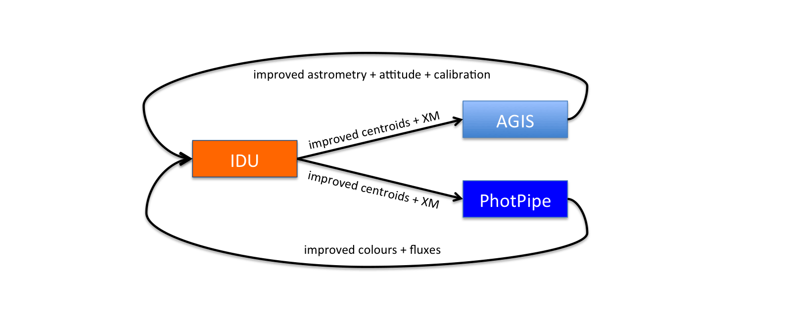
It represents the decisive overall iterative loop of the Gaia core processing expected to converge towards better and better astrometric solutions with time and the inclusion of increasingly more observation data as the mission progresses. Once the operational phase of the mission is concluded and no more input data arrive the looping will still have to continue for a while before the results settle. This is a consequence of the distributed and parallel nature of the processing in DPAC causing that not all systems can use the latest available and best possible input data at all times but possibly only older versions from the previous cycle. For Gaia DR1 no AGIS-PhotPipe-IDU loop was executed which is a known main weakness of this release (see Sect. 7 in Lindegren et al. 2016).

The PSF/LSF calibration in IDU will mainly benefit from AGIS’s improved geometric calibration and improved source colours from PhotPipe and the re-centroiding of observations will then ultimately lead to improved transit times. Note that when AGIS runs its calibration model (see Section 3.3) may include colour- and/or magnitude-dependent (COMA) terms in order to compute the best-possible astrometric solution. However, a subsequent IDU run will only evaluate the purely geometric port of the AGIS calibration since all COMA effects must be taken into account as part of the LSF/PSF calibration. Consequently, when AGIS processes the improved transit times the next time the corresponding COMA terms must be significantly reduced.

The second process in IDU with importance for AGIS is a new global crossmatch (XM) which assigns observations to sources in the working catalogue and also updates the working catalogue itself. This uses geometric calibration and improved attitude data from AGIS and generates a new version of the so-called match table that is a fundamental input to AGIS. The effect of a wrong-XM result from IDT on AGIS is that the set of observations belonging to the same physical source might be split among two or more real or spurious sources. As a result, the number of observations of the real source is lower than it ought to be and the astrometric solution for that source consequently weaker. If a source ends up with too few observations due to a wrong XM result, the astrometry for that source might be of very poor quality (large formal errors). This was the case for DR1 and as a result a number of sources have been filtered out. However, with only 14 month of mission data the number of observations per source might also be low (and the solution weak) just because the respective area of the sky has not been scanned very often yet. From the total number of objects eliminated from DR1 because of poor astrometric results it is unknown what fraction had XM problems.