10.13.4 Processing steps
The processing steps are:
-
•
time series segmentation,
-
•
outliers detection,
-
•
period search,
-
•
estimate of activity indexes,
-
•
best estimate of rotation period.
Segmentation
Segmentation of time series is required because the rotational modulation signal could be masked by the intrinsic evolution of spots and faculae, due to the evolution of the magnetic field intensity and topology. Ideally, the time series should be segmented in intervals shorter than the typical lifetime of spots and faculae (see the discussion in Distefano et al. 2023, for further details). In the Gaia case, this may lead to time-series segments with an insufficient number of measurements to detect the rotational modulation signal. A compromise has therefore to be found between the time span of the segment and the number of photometric measurements included in the segment. Since the sampling of the Gaia time series is strongly dependent on the ecliptic latitude, the code employs an ‘adaptive’ segmentation algorithm that takes the sampling of the different time series into account to estimate an optimal . This algorithm splits a given time series in marginally overlapping segments that satisfy the following requirement:
| (10.17) |
Outlier detection
In this step, outliers due to flaring events or to instrumental and calibration issues are detected and flagged. The rotational modulation analysis then considers the time series cleaned of such outliers. The outlier detection is based on the principle that, when the rotational modulation signal dominates the light curves, a linear correlation between magnitude and colour exists. For each segment, a robust linear regression is performed on the measurements versus . The measurements with the highest residuals from the model predictions are then rejected according to the criterion:
| (10.18) |
where and denote the mean and standard deviation of residuals, respectively. In some cases, this criterion can leave small residuals also for flare events that are significantly brighter and bluer than the mean values. In order to identify these measurements, the criterion
| (10.19) |
is also applied. All transits that satisfy at least one of Equations 10.18 and 10.19 are flagged as outliers and are not considered in the rotational modulation analysis.
Period search
The period search is performed in each segment and in the whole time series by running the Lomb-Scargle algorithm (Zechmeister and Kürster 2009) on the data (sub)set obtained after outlier rejection. The frequency interval in which the search is performed is (2, 3.2) d, with steps of d. The period with the highest amplitude in the periodogram is selected and its False Alarm Probability (FAP) is evaluated according to the formulation given by Baluev (2008). The period is flagged as significant if its FAP is less than the threshold value of 0.05 (see Lanzafame et al. 2018, for details on the threshold setting). If the FAP is less than 0.05, then the model given in Equation 10.16 is fitted to the photometric data.
Computation of activity indices
The variability amplitude in magnetically active stars is widely used as proxy of the stellar magnetic activity level. The code supplies two different magnetic activity indices for each segment and for each band. The first index is a trimmed peak-to-peak amplitude, defined as:
| (10.20) |
where and are the 5th and 95th percentiles, respectively, of the magnitude distribution in the segment and . The second index is the model peak-to-peak amplitude, defined as:
| (10.21) |
where and are the fit coefficients of Equation 10.16 and . The second index is given only when the fit model is available. Such an index is not explicitly given in the catalogue, but it can be computed from the fit coefficients.
Rotation period estimate
For a given star, the best estimate of the rotation period best_rotation_period is obtained by building the distribution of the periods detected in the different segments and by computing the mode of such a distribution, i.e., the period detected in the highest number of segments (see Distefano et al. 2023, for details on the algorithm developed to evaluate the mode). The periods used to compute the mode are only those associated with a FAP lower than the threshold value of 0.05 (see Section 10.13.4). The resulting period must then produce a good phase sampling of the folded light curve in at least one segment (where it was detected) and a sufficient reproducibility of the modulation with the model presented in Section 10.13.3 for all segments where it was detected. If these criteria are satisfied (see below), then the period is stored as best_rotation_period. If they are not, the second most frequent period is checked and so on. If no period satisfies these criteria, the star is not classified as a rotational modulation variable.
The phase sampling is parametrized through the Phase Coverage (PC) and the Maximum Phase Gap (MPG) parameters. The PC parameter is obtained by folding the light curve in a given segment according to the period detected in that segment. The folded segment is then divided into ten phase bins and PC is computed as the fraction of bins with at least one photometric measurement. The MPG parameter is computed as the maximum phase interval of the folded light curve that is not sampled by photometric points.
A coarse reproducibility of the modulation in the segment with the model in Section 10.13.3 is parametrized by the reduced chi-square of the best-fitting model and the ratio between the indices and , defined in Section 10.13.4. A value close to one and a low reduced chi-square suggest, in general, consistency between the folded light curve and the model.
When provided, the best_rotation_period satisfies the following criteria (see Distefano et al. 2023, for details on setting these threshold values):
-
1.
, for all the segments in which it has been detected,
-
2.
, for at least one of the segments in which it has been detected.
The segment satisfying the second requirement needs to be different from the whole time series.
Filtering of spurious candidates
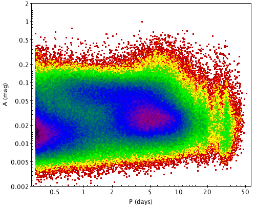
The quality requirements listed in Section 10.13.4 are more strict than those adopted in Gaia DR2, where the second requirement was more relaxed (the condition on was not present) and it could be satisfied by the whole time-series. The new requirements were enforced because of the spurious periods at 0.5, 18, 25, 32, and 49 d, which are visible in the period-amplitude diagram of the candidates. In Figures 10.30 and 10.31, we show the period-amplitude diagrams obtained with the Gaia DR2 and DR3 criteria, respectively. The periods used in the diagrams are given by best_rotation_period and the amplitudes originate from max_activity_index_g.
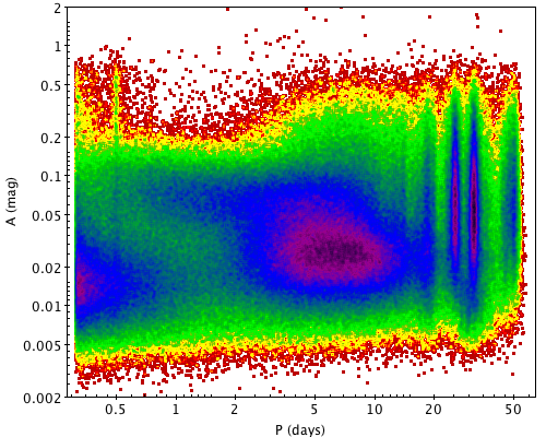
Though spurious periods are much less prominent in the preliminary candidates obtained with Gaia DR3 criteria, different features at about 0.5, 25, and 32 d are still visible in the diagram. The Gaia DR3 data set was therefore further cleaned by applying other quality criteria that evaluated the possibility that a given time series could be affected by a spurious signal. These quality criteria were based on the analysis of the image parameter determination (IPD) harmonic model time series and the per-transit-corrected-excess-flux time series. The analysis of the IPD harmonic model time series is discussed in detail in Holl et al. (2023a). The per-transit corrected excess flux is a quantity defined in Distefano et al. (2023) and is a measurement of the consistency between the , , fluxes measured during a given transit. Such a quantity is defined similarly to the corrected excess flux given in Riello et al. (2021) for the cumulative (per-source) photometry. The following additional quality criteria reduce the chance of candidates identified by spurious signals:
-
•
,
-
•
,
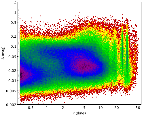
where is the Spearman correlation coefficient between the IPD harmonic models and the corresponding photometric measurements and is the Spearman correlation coefficient between the per-transit corrected excess fluxes and the corresponding photometric measurements. Both coefficients can be regarded as indicators of the possible presence of spurious signals, induced by the Gaia scan angle variation or instrumental effects in the time series (see discussions in Holl et al. 2023a; Distefano et al. 2023). In Figure 10.32, we show the period-amplitude diagram of rotational modulation candidates that satisfy all of the quality criteria.