10.8.5 Quality assessment and validation

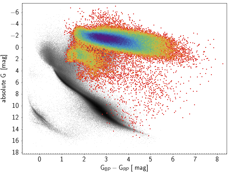
The observational Hertzsprung–Russell diagram of all LPV candidates with relative parallax uncertainties better than 15 % is shown in Figure 10.17. Almost all LPV candidates are found at the expected location in the diagram where asymptotic giant branch (AGB) stars stand. A small group of objects is also found at the blue side of the diagram below the AGB stars, close to the red clump brightness. These are likely red giant branch (RGB) stars.

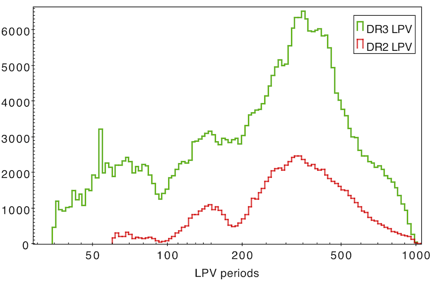
The distribution of the periods published in Gaia DR3 is shown by the green histogram in the left panel of Figure 10.18. It shows an overall distribution similar to what was published in the Gaia DR2 catalogue of LPV candidates, shown in red in the panel. Compared to the Gaia DR2 sample with published periods, the Gaia DR3 sample (a) contains many more sources and with amplitudes down to 0.1 mag (the lower limit was 0.2 mag in Gaia DR2), (b) contains periods down to 35 d (60 d in Gaia DR2), and (c) is based on observation durations of 34 months (22 months in Gaia DR2), thereby allowing many more detections with periods longer than 500 d.

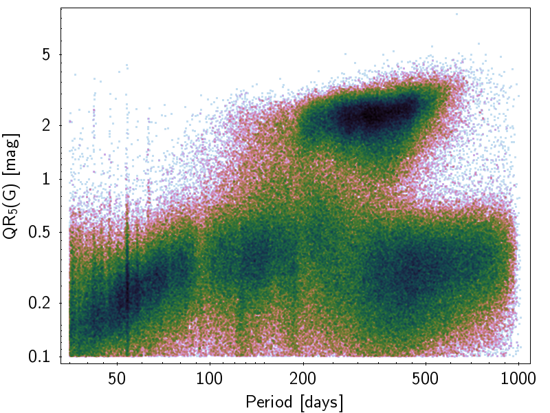
The period is shown against the 5–95 % trimmed range of $G$ in the right panel of Figure 10.18. The well-known trend of amplitude increasing with period is clearly visible on the short-period side of the diagram, while long secondary periods are visible at $P\gtrsim 300$ d. The group of points at the largest amplitudes is due to Mira variables. The figure also shows the presence of period aliases at short periods, visible from their vertical distributions at fixed values of the period.

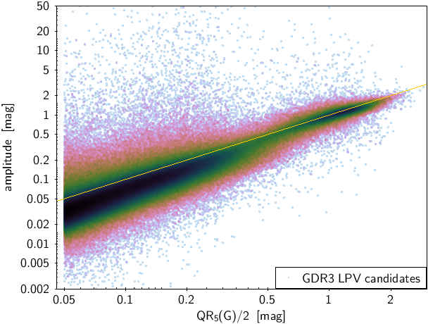
The model amplitudes published in the catalogue are shown versus half the 5–95 % trimmed range ${\mathrm{QR}}_5(G)$ of the $G$ light curves in Figure 10.19. For Miras (${\mathrm{QR}}_5(G)\gtrsim 1$), we see that the one-period model generally grasps well the full light curve amplitude, with model amplitudes about equal to half ${\mathrm{QR}}_5(G)$. This is expected from the fact that Miras pulsate in one mode. At smaller amplitudes, where semi-regular red giants are found, the one-period model only grasps part of the variability, as expected from the multi-periodic nature of semi-regulars. We therefore generally have the amplitude of the one-period model smaller than ${\mathrm{QR}}_5(G)$.

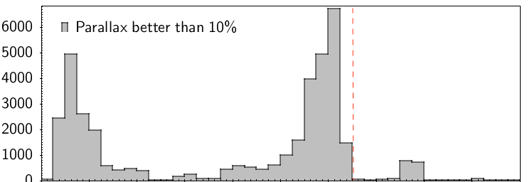
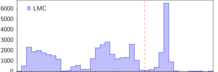
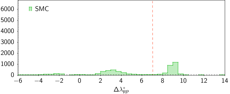
The histogram of the pseudo-wavelength separation $\mathrm{\Delta }{\lambda }_{\mathrm{RP}}^{\ast }$ between the two highest peaks in the RP spectra is shown in Figure 10.20 for three samples: Galactic candidates with relative parallax uncertainties better than 10 % (top panel), candidates in the Large Magellanic Cloud (LMC; middle panel), and candidates in the Small Magellanic Cloud (SMC; bottom panel). The LMC and SMC regions are defined with the same conditions on right ascension, declination, proper motion on the sky, and parallax as in Mowlavi et al. (2019). A good distinction is observed between O-rich candidates () and C-rich candidates ($\mathrm{\Delta }{\lambda }_{\mathrm{RP}}^{\ast }>7$). The distribution is a little more complex for candidates in the Galactic disc and bulge, probably due to the effect of extinction and/or higher metallicities (Lebzelter et al. 2023). In Figure 10.20, we also note the increased efficiency to produce C-stars in lower metallicity environments: the fraction of C-stars is the lowest in the solar-metallicity Galactic sample shown in the top panel and largest in the SMC shown in the bottom panel.

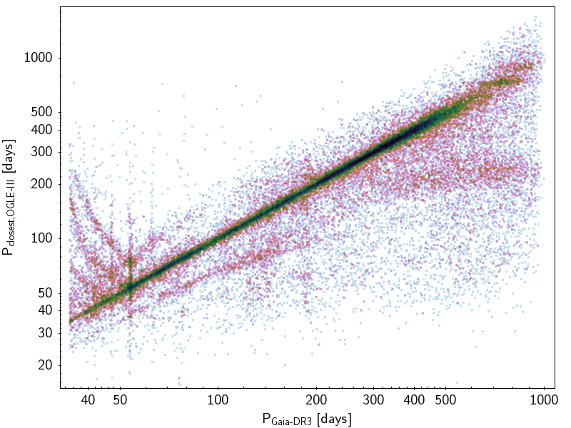
The Gaia DR3 periods are compared to the periods obtained by the Optical Gravitational Lensing Experiment (OGLE) for LPVs in the Magellanic Clouds and Galactic bulge. We cross-match our candidates with the OGLE-III catalogues (Soszyński et al. 2009a, 2011, 2013) within 2 arcsec. Figure 10.21 compares, for each matched source, the Gaia DR3 period with the closest OGLE-III period among the primary, secondary, and tertiary periods. The Gaia DR3 periods are within 10 % of the closest OGLE-III period for about 55 % of the matched sources. In about half of the cases, the period detected by Gaia corresponds to the primary period from OGLE-III, while the remaining cases are roughly evenly split between secondary and tertiary periods.

The distinction between C-rich and O-rich stars has been confirmed on a statistical basis by comparison with M- and C-stars classified from the ground. S-type stars (O-rich giants with intermediate properties between M- and C-types, and showing spectral signatures of s-process elements) and hot C-stars cannot be safely identified with the help of this criterion. In addition, sources with $\mathrm{\Delta }{\lambda }_{\mathrm{RP}}^{\ast }$ values larger than 10 (see Figure 10.20) are most probably O-rich stars, and therefore misclassified as C-rich stars in the Gaia DR3 catalogue. For more details and an improved criterion (including colour-dependence), we refer to Lebzelter et al. (2023).

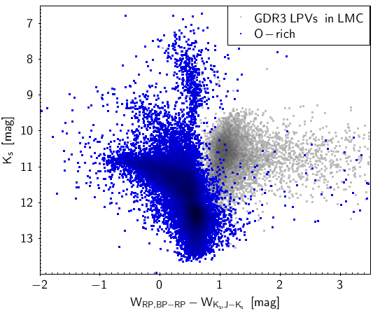
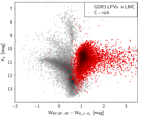
An additional validation of the C-rich classification is presented in Figure 10.22, which combines Gaia and 2MASS data (Skrutskie et al. 2006). The figure shows the Gaia-2MASS diagram of the LPV candidates in the LMC, plotting the 2MASS $K_s$ magnitude versus the difference between the $G_{\mathrm{RP}}$ Wesenheit index ($W_{RP,BP-RP}=G_{\mathrm{RP}}-1.3(G_{\mathrm{BP}}-G_{\mathrm{RP}})$) and the $W_{K_s,J-K_s}$ Wesenheit index ($W_{K_s,J-K_s}=K_s-0.686(J-K_s)$). O-rich LPVs (in blue in the left panel) are distributed in the left part of the diagram, while C-rich LPVs (in red in the right panel) are distributed in the right part of the diagram, as expected from the study of Lebzelter et al. (2018).