5.1 Introduction
5.1.1 Overview
Author(s): Dafydd W. Evans
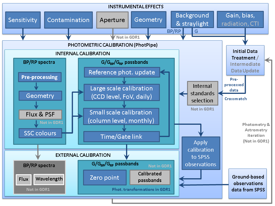
Figure 5.1 from Carrasco et al. (2016) shows an overview of the data processing for photometry, the elements of which are further described in the following sections.
5.1.2 Notations, nomenclature, and definitions
Author(s): Francesca De Angeli
The following list of concept might be useful for a good understanding of the content of this chapter:
-
•
CCD transit, the transit of a source across one single CCD.
-
•
FoV transit, field-of-view transit, the complete transit of a source across the focal plane, this may include one SM transit, 9 (or 8) CCD transits, one BP transit and one RP transit. The RVS CCD transit is irrelevant for this chapter.
-
•
Source catalogue, the catalogue formed by all sources observed by Gaia. This is updated at each cycle. The catalogue used in cycle N is the one generated by the MDB Integrator at the end of cycle N-1.
5.1.3 Spectral Shape Coefficients
Author(s): Josep Manel Carrasco, Floor van Leeuwen
Colour information of the observed sources is an essential element of the photometric calibration. The colour information required is obtained from the low-resolution spectra from the BP and RP spectro-photometers from which are derived the so-called spectral-shape coefficients (SSC). The wavelength ranges of the SSC rectangular bands are given in Table 5.1. Although they fulfil the same role, the SSCs are not strictly pass bands. The along-scan smearing from the line-spread function (LSF) means that the SSC boundaries are fuzzy, and depend on issues such as the exact positioning of the spectrum with respect to the pixel binning of the spectrum, the local dispersion function and small variations in the along- and across-scan rotation rates. Still, implementation has shown improved performances of the calibrations compared to using the ratio of integrated BP and RP fluxes.
Figure 5.2 shows the location of the SSC bands in the data space compared to the BP and RP simulated spectra for a sample of template stellar spectra covering the effective temperature range from to K. Figure 5.3 shows the expected SSC dependency with the colour of the star for a data set of simulated BP and RP spectra covering a wide range of spectral types (Carrasco et al. 2016).
| Photometer | SSC id | range (nm) |
| BP | 0 | [328, 433] |
| 1 | [433, 502] | |
| 2 | [502, 559] | |
| 3 | [559, 720] | |
| RP | 4 | [618, 719] |
| 5 | [719, 785] | |
| 6 | [785, 863] | |
| 7 | [863, 1042] |


5.1.4 Reference System
Author(s): Dafydd W. Evans
The basic principles behind the photometric calibrations is that they are split between an internal and external component. The internal calibrations bring all observations onto the same reference system, while the external calibrations provide the transformation between this internal system and an absolute one that can be interpreted physically. This general principle is applied to both the flux photometry and the BP/RP spectra. The models used for the internal calibration are described in Section 5.3.3. The external calibration model is described in Section 5.3.4.
For the internal calibration of the fluxes (G-band, integrated BP/RP and extracted SSC fluxes, Section 5.1.3), the reference system needs to be set up. No external data is used in the generation of these reference fluxes. The reason for only using data from the satellite is that if ground-based data is used, seasonal and hemispheric systematic effects can be introduced into the system. Also, Gaia has the potential to provide data that has better uncertainties and sky coverage than any current survey.
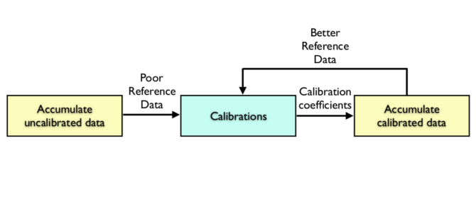
The internal calibration is carried out in a bootstrap manner illustrated in Figure 5.4. Initially, the reference fluxes are generated for each source by accumulating all the raw (uncalibrated) fluxes and generating weighted mean values. Using these as an initial reference, calibrations are carried out. There then follows an iterative loop where the calibrations are used in accumulating calibrated fluxes to generate a better set of reference fluxes and the calibrations repeated.
This method converges since the observations for the sources have different calibrations applied to them and that each calibration is carried out with different sources. Given that there is good mixing between the calibrations and sources, i.e., more than half of the sources are observed in two or more configurations (CCD, Gate, FoV, …), this process should converge quickly. Conversely, if there is no mixing between sources and calibrations, multiple photometric systems could form, e.g., two sets of sources are observed in different configurations, each needing their own set of calibrations, would result in two independent photometric systems.
In general, this is not the case with Gaia, but there are cases in which there is poor mixing, where additional calibrations are needed to speed up the convergence. These calibrations are referred to as link calibrations since they link the photometric systems between different configurations. The two identified link calibrations are:
-
•
Time Link Calibration. During the early stages of the mission, Gaia observed in a configuration known as Ecliptic Pole Scanning Law (see Section 1.3.2). A consequence of this was that a significant fraction of sources observed was mostly observed during that specific time periods. This was also the period when the contamination of the mirrors was worst and evolving most rapidly (Section 1.3.3). Including these data in the calibrations caused the early attempts at defining the reference system to show a linear trend with time in the residuals. The initial accumulation of the raw fluxes had imprinted the contamination signal into the reference system. The Time Link Calibration uses differential measurements to largely remove this signal from the raw data without the need for an external set of reference fluxes.
-
•
Gate/Window Class Link Calibration. The determination of the gate and window class is used for an observation is made on-board using an instantaneous magnitude determination. If this is accurate and the source is constant, there will be very poor mixing since a source will almost always be observed with the same gate and window class configuration and thus be associated with the same set of calibrations. Although, the accuracy is poor (0.3–0.5 mag) at the bright end (), it is sufficiently accurate to cause problems for setting up the photometric reference system fainter than this. The Gate/Window Class Link Calibration uses differential measurements to link these configurations prior to the initial raw flux accumulation.
Further details on these link calibrations can be found in Section 5.3.3.
A similar scheme is envisioned for the instrument calibration of the BP/RP spectra in that there will be an iterative loop between the instrument calibration and the source update process which provides the reference spectra.
For more details on the photometric reference system, see Carrasco et al. (2016).