5.4 Photometric processing 5.4 Photometric processing 5.4.2 Validation

5.4.1 Calibration

Author(s): G. Busso, P. Montegriffo

As explained in Section 5.1.2, the calibration is split in internal calibration, using only Gaia observations to bring all data in the same Gaia reference system, and external calibration, comparing the internally calibrated fluxes of standard stars with their corresponding absolute fluxes that can be interpreted physically.

Internal Calibration

Author(s): G. Busso

Section 1.1.3 describes the complexity of the Gaia instrument, highlighting the fact that there are many configurations with which an observation is acquired (Field of view, CCD strip, CCD row, window class, gate). The CCD response might also vary with the AC position in the CCD. Furthermore, because of how the mission is carried out, the response of the instruments is time dependent. It is then not possible to compare observations with different configurations, obtained at different times, unless they are first calibrated to an average photometric system. This is the fundamental job of the internal calibration, that is to determine the variation of the global response of the photometric instrument over the mission and between different configurations. For a complete description of the photometric calibration models, please refer to Carrasco et al. (2016) and Riello et al. (2020).

The internal calibration is split into Small Scale (SS) calibrations, modelling the fluctuations of the sensitivity at pixel level, and Large Scale calibrations, which accounts for variations in the mean response at the CCD level and for every FoV. The SS calibration duration must be long enough to accumulate sufficient data to be able to calibrate the response of a single pixel column, while the LS calibration needs to be able to reflect the rapid (and sometimes discontinous, for instance in case of decontamination or refocus) changes of the overall instrument response, hence its duration is much shorter.

Both SS and LS calibrations are in principle described by a n-th degree polynomial function depending on a colour term, to take into account that the response variations are wavelength dependent, and on the position on the CCD. The colour information comes from the BP/RP spectra, either as $G_{\mathrm{BP}}-G_{\mathrm{RP}}$ or as SSCs (see Section 5.1.1).

In Gaia DR2, the LS calibration was based on the SSCs calculated on raw spectra (see Riello et al. (2018)). These SSCs were then calibrated in the same way as the $G$ , $G_{\rm BP}$ and $G_{\rm RP}$ epoch photometry and then accumulated to obtain for every source a set of mean SSCs which were first normalised and then used to in the calibrations. This colour information was updated at every iteration, causing some fluctuations in the process of building the photometric system. In Gaia EDR3 instead the LS calibration is based on the SSCs calculated on the internally calibrated mean spectra, keeping the processing more stable. The SSCs are not normalised but they are combined in flux ratios, creating pseudo-colours. A further improvement is also the introduction of a flux loss term, taking into account that the transit window’s limited size hinders the acquisition of the total flux, which affects 1D observations.

The SS calibration model is the same as in Gaia DR2, that is a simple zero-point covering a group of 4 pixel columns. For more details on the selection of the calibrators and the definition of the LS and SS models, please refer to Riello et al. (2020). In the following the steps followed to obtain the calibrations are explained.

The derivation of the reference fluxes was carried out on a restricted time period where the effects of contamination by water ice on the mirrors and CCDs (Gaia Collaboration et al. 2016b) was at a lowest level and the instrument was the most stable (see Fig. 5 in Riello et al. (2020)). This period was long enough for the scanning law to ensure that the entire sky was covered multiple times and it is referred to as the INIT period. In this time period, a group of calibrators were extracted: the selection was based on a minimum number of observations per source, and on a flattened distribution of colour ( $-1.0<G_{\mathrm{BP}}-G_{\mathrm{RP}}<6.0$ ) and magnitude ( $5.0<G<19.0$ ). Also all stars used for the external calibration and the passband validation (see Section 5.6) were included.

Using the full link–calibrated fluxes, a new set of reference fluxes were accumulated. These were then used in the first of the large-scale calibrations. These generally have a time scope of one day. This calibration has the biggest effect on reducing the overall systematics in the fluxes.

The large-scale calibration and accumulation processes are then iterated until the calibrations are reasonably stable. This is assessed using an L1 norm metric as described in Evans et al. (2017). For Gaia EDR3, 20 iterations were carried out.

The small-scale calibrations were then calculated using the large-scale-calibrated reference fluxes. The time scope for the small-scale calibrations covered the entire initialisation period. Two sets of iterations were then carried out between the large and small-scale calibrations to ensure that the minimum standard deviations for the solutions were achieved and that these calibrations were stable. No accumulation process was carried out between these iterations, i.e., the reference fluxes remained the same throughout this process. Using these large and small-scale calibrations, the source photometry for the INIT period was derived.

This was used to generate a series of large and small-scale calibrations covering the entire period considered for Gaia EDR3. The time scopes for the large-scale calibrations was one day, as in the initialization of the reference system, and for the small-scale calibrations three time scopes were used. These calibrations were then applied to calibrate the epoch fluxes, which were accumulated to generate the weighted-mean fluxes that are released in the catalogue.

The sources that were calibrated with the described procedure are referred to as $g o l d$ sources, where all 8 SSCs are available. Gold sources were also used to estimate empirical relationships between $G$ , $G_{\rm BP}$ and $G_{\rm RP}$ to be used in case, either for BP or RP, some or all SSCs are missing. In this case the sources are referred to as $s i l v e r$ . In the worst case, when all SSCs are missing from both BP and RP, the sources are referred to as $b r o n z e$ and they are calibrated using default SSCs. The same approach was adopted in Gaia DR2 for bronze processing.

Accumulations

Author(s): Dafydd W. Evans

As part of the iterations to establish the photometric reference system, accumulations are used to determine an average flux value (see Figure 5.4). The accumulations refer to weighted summations that are carried out for each source of their individual flux values. The three used in Gaia DR2 are $\sum_{k}w_{k}$ , $\sum_{k}I_{sk}w_{k}$ and $\sum_{k}I_{sk}^{2}w_{k}$ where $I_{sk}$ is the individual flux measurement for observation $k$ and source $s$ and $w_{k}=1/\sigma_{k}^{2}$ is the weight used. $\sigma_{k}$ is the error on the flux quoted by the IPD, see Section 3.3.5). Note that the same notation as Carrasco et al. (2016) is used to avoid confusion.

As for the previous releases, inverse variance weighted mean values are used for the averages. Weighted means were chosen since the fluxes are heteroscedastic, i.e., the flux errors vary depending on the gate and window class configuration of the observation. The most significant configuration is gating since the effective exposure time of the observation is determined by this. In addition to this, sigma clipping has been introduced for the second data release. This is needed since the flux distribution can be non-Gaussian due to the presence of outliers. The sigma value for this filtering is determined from a robust estimate of the scatter of the observed fluxes. Median absolute deviation was used for this and a five sigma clipping was done. The reasons for measuring the value used for the sigma rather than using the formal errors from the IPD are that the errors can also be outlier in nature and that the source could be variable. In the latter case, too many observations would be filtered out if the formal errors were used in the sigma clipping.

As mentioned above, the weighting scheme used is the inverse variance $w_{k}$ . Thus, after sigma clipping has been applied, the weighted mean flux for each source, $\overline{I_{s}}$ , is given by

\overline{I_{s}}=\frac{\sum_{k}I_{sk}w_{k}}{\sum_{k}w_{k}}

(5.8)

Since the errors quoted for the flux quantities derived from the IPD do not fully account for modelling errors, they will be a slight underestimate of the observed error distribution. An example of such modelling errors is due to a simplified PSF/LSF being used in IPD. For Gaia DR2, the PSF/LSF did not account for dependencies on time nor colour. These dependencies will gradually be added in future processing cycles. To account for these modelling errors, the intrinsic scatter of the fluxes is used in the error calculation in the same way as used for the mean photometry of the Hipparcos catalogue ESA (1997):

\sigma_{\overline{I_{s}}}=\sqrt{\frac{\sum_{k}I_{sk}^{2}w_{k}-\overline{I_{s}}% ^{2}\sum_{k}w_{k}}{N_{\rm obs}-1}}\cdot\frac{1}{\sqrt{\sum_{k}w_{k}}}

(5.9)

where $N_{\rm obs}$ is the number of CCD observations. The weighted mean flux and error given in Equation 5.8 and Equation 5.9 are the quantities used in the photometric calibrations as the reference fluxes.

Other useful quantities can be derived from the accumulations that can help in detecting variables or determining whether the calibrations are at the photon noise level or not.

The reduced $\chi^{2}$ , sometimes known as the unit weight variance, is given by

\frac{\chi^{2}}{\nu}=\frac{\chi^{2}}{{N_{\rm obs}-1}}=\frac{{\sum_{k}I_{sk}^{2% }w_{k}-\overline{I_{s}}^{2}\sum_{k}w_{k}}}{{N_{\rm obs}-1}}

(5.10)

where $\nu$ is the degrees of freedom. The $\chi^{2}$ can be used to provide a quantity known as a P-value:

P=Q(\frac{\nu}{2},\frac{\chi^{2}}{2})

(5.11)

where Q is an incomplete gamma function (Press et al. 1993). P-values can be used to identify variable sources if the quoted errors are reliable and the calibrations have accounted for all systematic errors. For constant sources the distribution of the P-values will be flat between 0 and 1, whereas for variable sources it is strongly skewed towards 0. The advantage of P-values is that they are easier to interpret directly in comparison to the reduced $\chi^{2}$ , and that the number of false positives from any variability detection limit is simply this limit multiplied by the number of sources. However, due to the underestimation of the individual flux errors from the IPD, the P-values for almost all sources is very close to 0 and thus are viewed as variable from this measure. It should be reiterated that, although no rescaling is carried out on the individual flux errors, the measurement of the error on the weighted mean flux, Equation 5.9, since it accounts for the scatter in the data for each source, is a realistic estimation of the error and is thus not underestimated.

Another way of estimating the additional scatter caused by variability is given by Equation 87 of van Leeuwen (1997) (page 349). This simplifies the variability as a sinusoidal variation and calculates an excess noise quantity:

A=\sqrt{\frac{2(\chi^{2}-\nu)}{\sum_{k}w_{k}}}

(5.12)

When calculating this quantity, checks must be made that the numerator is not negative. If this is the case, then the source is unlikely to be variable and no excess noise is measurable.

External Calibration

Author(s): Paolo Montegriffo

The main objectives of the external calibration are to provide for each of the filters $G$ , $G_{\rm BP}$ and $G_{\rm RP}$ the current shape of the passband and the corresponding zero points to allow for the transformation of internally calibrated mean fluxes into magnitudes.

To this purpose a model for the passband is generally used, whose shape depends on a number of adjustable parameters: given a set of sources of known SED, the free parameters can be best-fitted to minimise the differences between observed and synthetic fluxes. For Gaia DR2 the passbands were derived in this way using the catalogue of SPSSs described in Section 5.6. However, the Gaia DR2 processing has shown that by the use of the SPSSs alone the shape of the filters cannot be constrained with sufficient accuracy, especially where sharp features such as steep cut-ons and cut-offs are present as in the BP and RP case. This is due both to the relatively small number of available calibrators, and also because the SPSS SEDs span necessarily only a subspace of all possible spectra shapes, and hence only the parallel components of the filter can be usefully constrained ((Weiler et al. 2018)). This has an impact on the integrated photometry because a significant amount of information is lost in the wavelength integration process. For this reason in Gaia DR3 a new strategy has been adopted, where the two major novelties are:

•

for $G_{\rm BP}$ and $G_{\rm RP}$ no attempt is made to fit the cut-ons and cut-offs within the processing of integrated photometry, but rather their current positions and shapes are taken from the XP instrument model processing, that will be described in detail in the Gaia DR3 documentation;
•

the set of calibrators has been expanded to include a huge number of sources ( $N\gtrsim 100000$ ) whose SEDs were obtained by externally calibrated Gaia XP spectra. Note however that, as described in Section 5.3.5, the absolute scale of XP spectra is based on the SPSS, so the reference absolute flux scale does not change because of this choice.

Passbands

The internally calibrated integrated flux $n_{p}$ for a source in a Gaia filter is given as an accumulated flux in unit of $photo\textrm{-}electrons~{}s^{-1}$ . The model to link this flux to the source own photon flux distribution is:

n_{p}=P\int\,n_{p}(\lambda)\,S(\lambda)\,{\rm d}\lambda

(5.13)

where $P$ represents the telescope pupil area and $S(\lambda)$ is the system overall response function that includes the scaling factor to convert from $p h o t o n s$ to $photo\textrm{-}electrons$ .

This response function represents the passband and is modelled as the product of some reference response function $R_{*}(\lambda)$ and a parametric function based on a linear combination of a suitable set of orthogonal basis functions $B_{i}(\lambda)$ :

S(\lambda)=R_{*}(\lambda)\times\exp\left(\sum_{i=0}^{n_{R}}r_{i}\;B_{i}(% \lambda)\right)

(5.14)

The basis functions used for the Gaia DR3 processing are Legendre polynomials. The adopted reference response function for the $G$ band differs from that adopted for the $G_{\rm BP}$ and $G_{\rm RP}$ cases: in the first case $R_{*}(\lambda)$ is the nominal pre-launch response described in Jordi et al. (2010) and is computed as

R_{G}(\lambda)=T_{0}(\lambda)\,\rho_{att}(\lambda)\,Q(\lambda)

(5.15)

where

1.

$T_{0}(\lambda)$ is the telescope (mirrors) reflectivity;
2.

$\rho_{att}(\lambda)$ is the attenuation due to rugosity (small-scale variations in smoothness of the surface) and molecular contamination of the mirrors;
3.

$Q(\lambda)$ is the CCD QE;

All these quantities were initially measured by Airbus DS during on-ground laboratory test campaigns.

For $G_{\rm BP}$ and $G_{\rm RP}$ the reference response $R_{*}(\lambda)$ is a cubic spline interpolation on a 1nm fine grid lookup table derived from the XP instrument model (see Section 5.3.5).

Provided that the reference response function is non negative, the exponential form of the parametric function in Equation 5.14 guarantees the non negativity of the passband $S(\lambda)$ . To least square fit the $r_{i}$ parameters, the partial derivatives of the model with respect to the parameters are also needed:

\frac{\partial S(\lambda)}{\partial r_{i}}=R_{*}(\lambda)\times\exp\left(\sum_% {i=0}^{n_{R}}r_{i}\;B_{i}(\lambda)\right)\times B_{i}(\lambda)

(5.16)

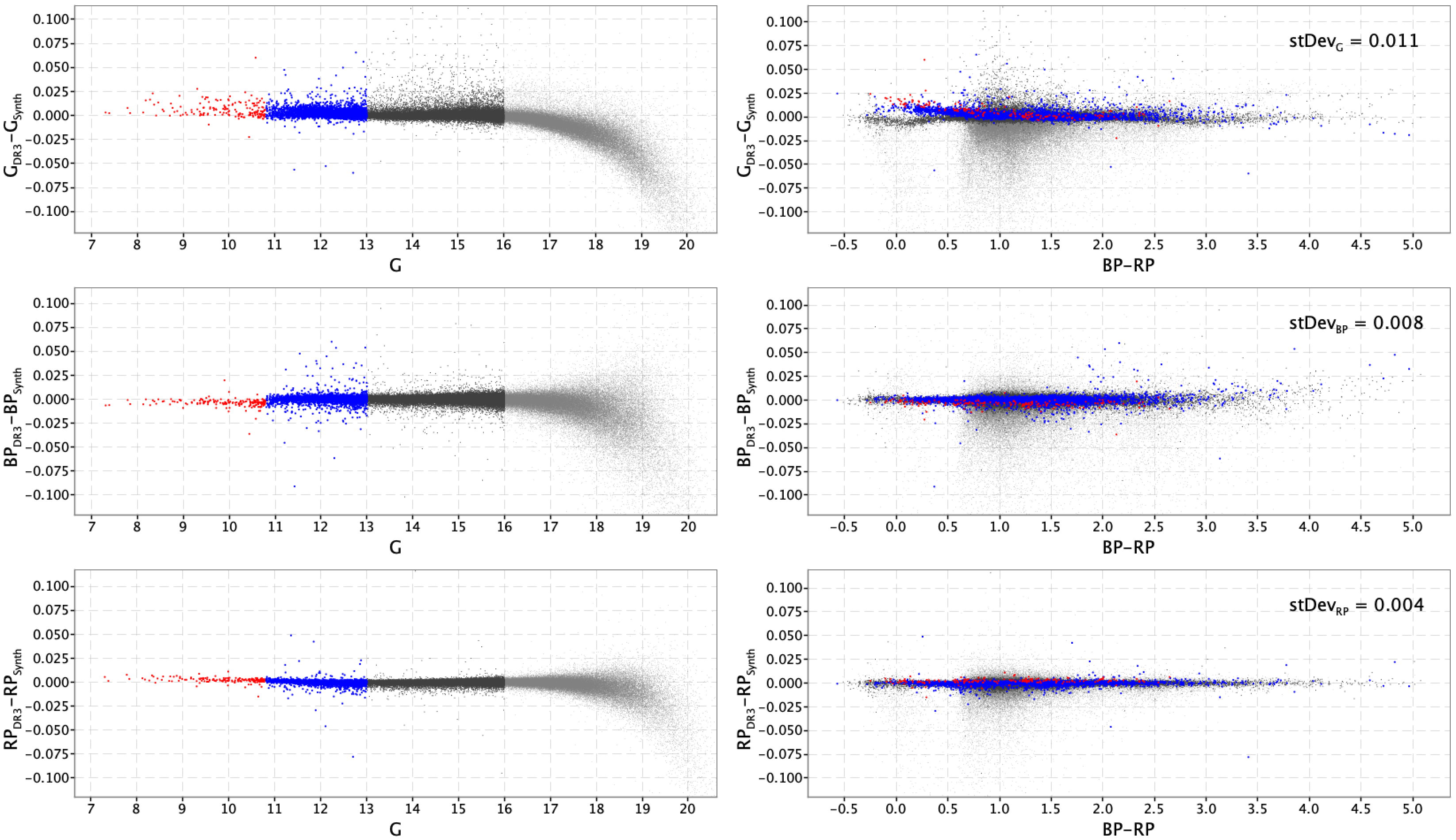
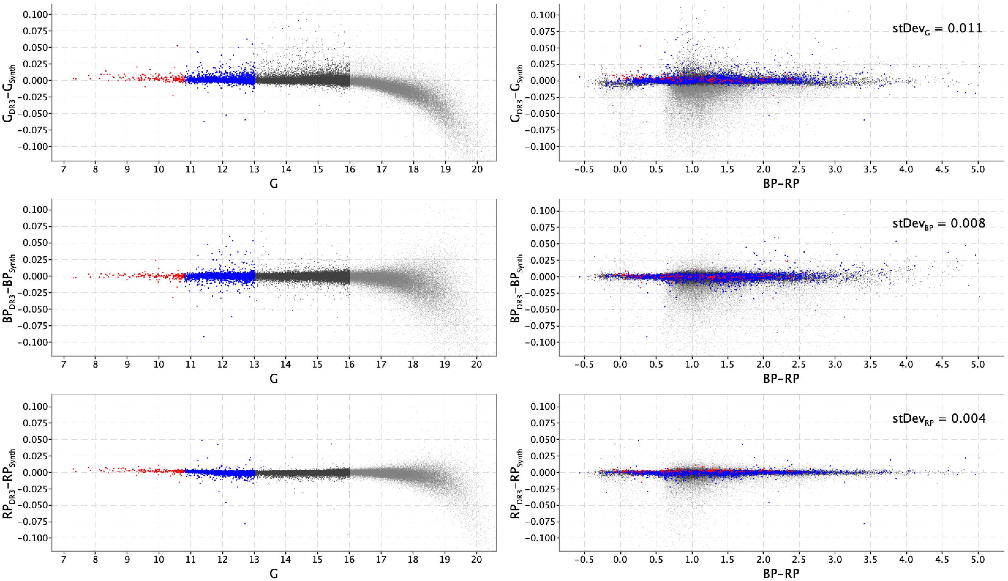
Figure 5.9: Residuals between Gaia DR3 and synthetic magnitudes computed on a sample of $\sim 100000$ SEDs obtained from externally calibrated XP spectra for $G$ (top), $G_{\rm BP}$ (middle), $G_{\rm RP}$ (bottom) as a function of $G$ magnitudes (left) and $G_{\mathrm{BP}}-G_{\mathrm{RP}}$ colours (right). Synthetic magnitudes have been computed with a preliminary set of passbands.

Figure 5.9 shows the residuals obtained with a preliminary set of passbands between the Gaia DR3 and synthetic magnitudes for the calibrators sample; residuals are shown as a function of magnitude on the left panels and of $G_{\mathrm{BP}}-G_{\mathrm{RP}}$ colour on the right panels. Different colours are set for $G<10.8$ (red), $10.8<G<13$ (blue), $13<G<16$ (dark grey) and $G>16$ (light grey). A few issues are clearly visible:

•

in $G$ there is a colour term affecting sources brighter than $G=13$ and bluer than $G_{\mathrm{BP}}-G_{\mathrm{RP}}\simeq 1.0$ ;
•

in $G_{\rm BP}$ there is a small jump at $G\simeq 10.8$ , possibly a residual effect of a gate not properly calibrated;
•

a hockey stick feature is visible in all three passbands for sources fainter than $G\simeq 16.5$ , possibly caused by some bias in the background either in the integrated photometry or in the XP spectra.

Magnitudes $G=13$ and $G=16$ correspond to Window Class changes, so a possible explanation for the $G$ colour term for bright sources may be that the internal calibration for these did not successfully converge on the same photometric system as the fainter ones, a situation similar to that seen in Gaia DR2 for the BP case (see Maíz Apellániz and Weiler (2018)). Moreover, the fact that this issue is not visible in the $G_{\rm BP}$ and $G_{\rm RP}$ cases suggests that the effect is due to problems in the integrated photometry of the $G$ band rather than to unidentified problems affecting the calibration of XP spectra. Rather than computing two different passbands to characterise the photometric systems of bright and faint sources, a correction factor for $G$ fluxes was calculated and applied to the data (mean and epoch photometry) before photometry was exported to the MDB, so that the whole dataset can be described with one passband. To derive this $G$ correction relation two intermediate passbands were computed, one for sources brighter than $G=13$ and the other for sources with $13<G<16$ , then by comparing synthetic fluxes $g$ computed through the two passbands the polynomial relation was fitted as a function of the $bp/rp$ flux ratio:

g_{corr}=g\times\sum_{i=0}^{3}c_{i}\;\left(\frac{bp}{rp}\right)^{i}

(5.17)

with $c=\{0.993829660,~{}0.0118274517,~{}-0.00197201647,~{}2.25361886E-4\}$ . This correction has been applied only to sources with $G<13$ and $G_{\mathrm{BP}}-G_{\mathrm{RP}}<1.1$ . A similar approach has been adopted also to remove the $G_{\rm BP}$ jump:

bp_{corr}=bp\times 10^{-0.4\;BP_{offset}}

(5.18)

with $BP_{offset}=0.00376309633$ for $G<10.8$ .

Figure 5.10: Top left: Colour-Magnitude diagram for all-sky sources with the uncorrected fluxes; top right: the same diagram after a sudden correction: a gap appears in the data; bottom left: the same diagram after a gradual application of the correction; bottom right: histograms of the magnitudes before (red) and after (green) correction.

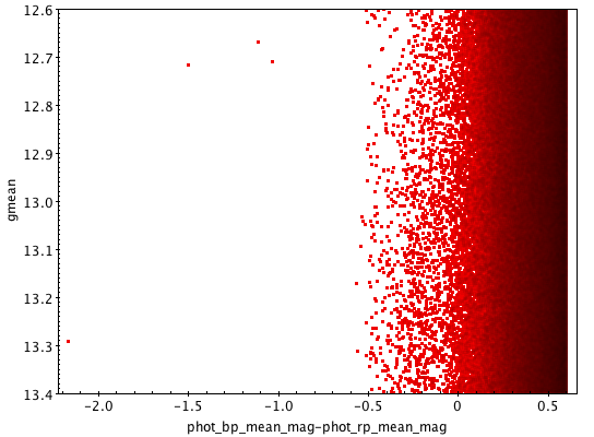
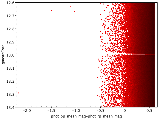
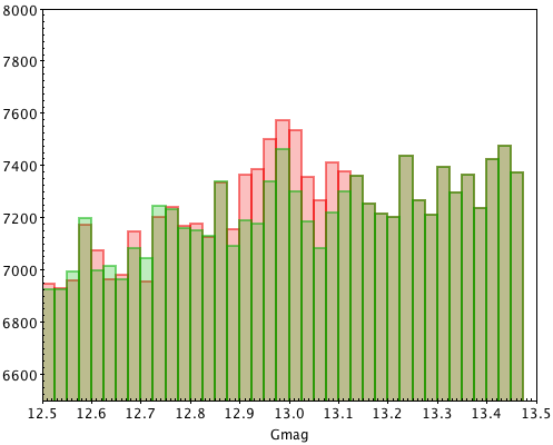
To avoid the creation of artefacts in the data, such as visible gaps in colour-magnitude diagrams that would be produced by a sudden correction as that of Equation 5.17, the correction was applied gradually ( $\pm 10\%$ in flux around $G=13$ ). Figure 5.10 illustrates the case: the top left panel shows the all-sky colour-magnitude diagram around $G=13$ ; in the top right panel a gap is clearly visible after a sudden correction was applied; the bottom left panel shows the same diagram after the correction was applied gradually: no gap is seen in the distribution. Finally the plot in the bottom right panel compares the histograms of the magnitudes before (red) and after (green) correction. It has been suggested that the over-density around $G=13$ might be a result of this issue and not of astrophysical origin; the correction alleviates this feature.

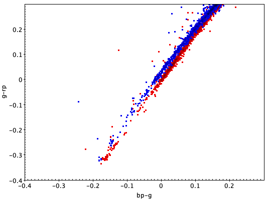
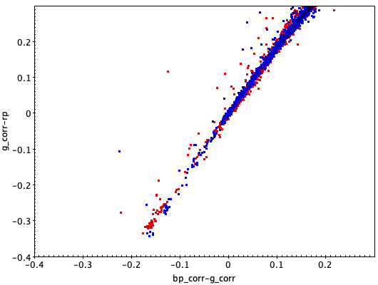
Figure 5.11: Colour-colour diagram of high galactic latitude sources with $12<G<13$ (blue dots) and $13<G<14$ (red dots).

As a further support to check the accuracy of the suggested relations, Figure 5.11 shows the effect of the corrections on the colour-colour diagram $G$ - $G_{\rm RP}$ vs. $G_{\rm BP}$ - $G$ of a sample of high latitude stars with $12<G<13$ (blue dots) and $13<G<14$ (red dots): the uncorrected diagram on the left shows clearly an un-physical double sequence that almost disappears after the correction is applied. Since the data used for the plot rely entirely on integrated photometry, this confirms that the $G$ colour term is due to problems in the photometry and not in the calibrated XP spectra.

The final passbands have been then computed using only sources in the range $13<G<16$ , $11<G<16.5$ and $G<16.5$ respectively for $G$ , $G_{\rm BP}$ and $G_{\rm RP}$ ; in all cases 3 Legendre polynomials have been used in Equation 5.14 to model the passbands. Figure 5.12 shows the final residuals between observed and synthetic magnitudes for the whole set of calibrators. Residuals are quite flat in colour and rms errors range from $\sim 0.01$ mag for $G$ to less than $\sim 0.005$ mag for the $G_{\rm RP}$ case.

Figure 5.12: Residuals between Gaia DR3 and synthetic magnitudes obtained with the final passbands.

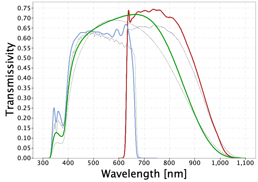
The Gaia DR3 passbands are shown in Figure 5.13, nominal pre-launch passbands are plotted for comparison.

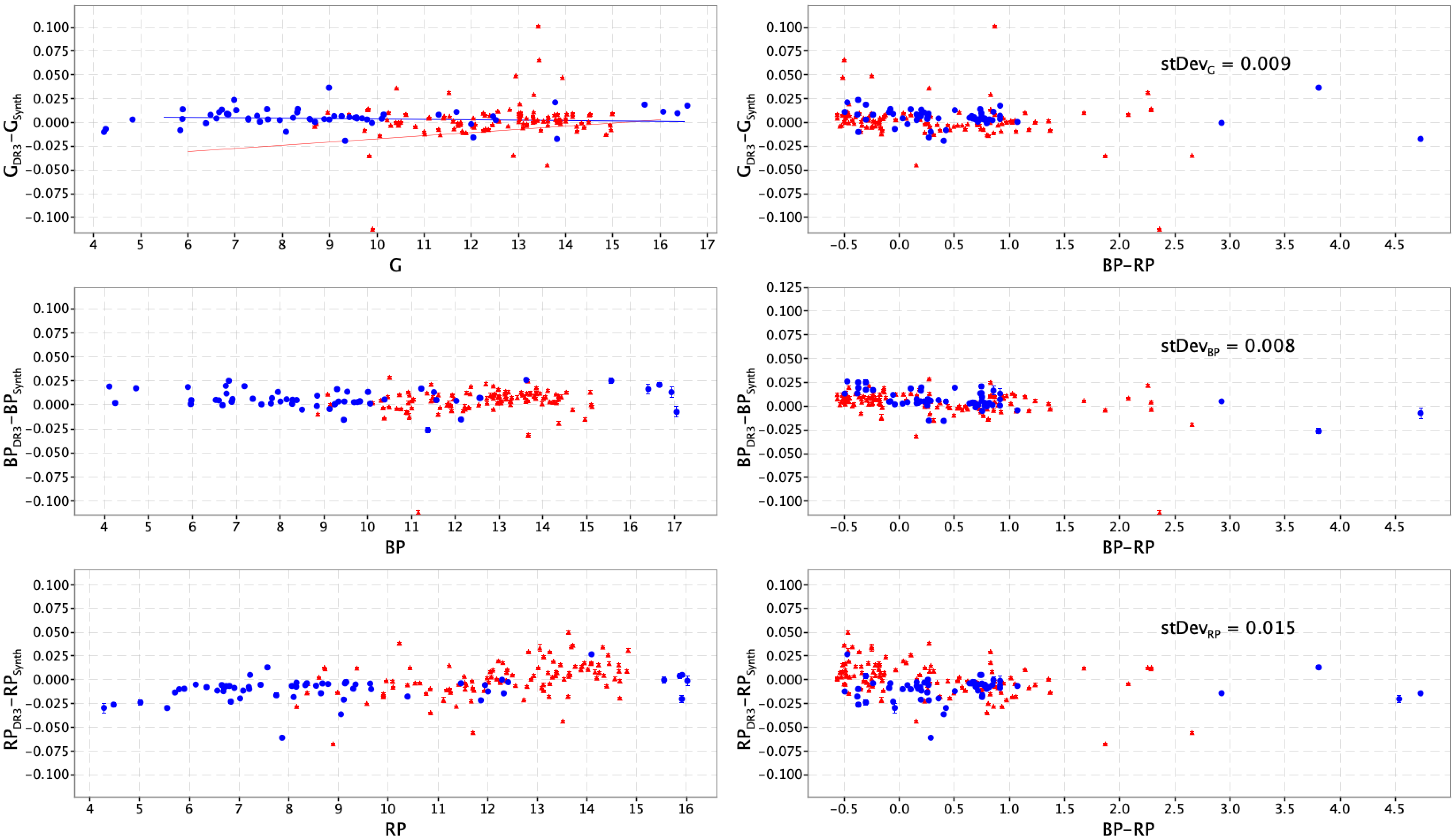
Figure 5.13: $G$ (green), $G_{\rm BP}$ (blue) and $G_{\rm RP}$ (red) passband for Gaia EDR3 photometric system; grey curves represent nominal pre-launch curves

Figure 5.14: Residuals between Gaia DR3 and synthetic magnitudes for SPSS (red dots) and PVL sources (blue dots). Unlike previous plots, synthetic photometry has been computed on independent SEDs coming from ground or space based observations.

Finally, as a further validation the residuals between observed and synthetic magnitudes for SPSS and PVL catalogues were computed (see Section 5.6): the difference from Figure 5.12 is that in this case the synthetic photometry is computed on independent SEDs from ground or space based observations. The red line visible in the top left panel represents the relation given by Casagrande and VandenBerg (2018) modelling the residuals affecting Gaia DR2 $G$ photometry. The blue line represents a fit to the current data and clearly shows the improvements made by Gaia DR3 calibrations. Small offsets are visible between SPSS (red dots) and PVL (blue dots) up to $\sim 0.01-0.02$ mag in the RP case: the SPSS calibration is tied to the CALSPEC system available in 2013-2015. CALSPEC underwent a major revision of its flux scale in 2017-2019 with an offset of the order of $1\%$ (i.e., 0.01 mag approx). This should explain the average observed offset and is not worrisome: CALSPEC and Landolt also disagree at the $1\%$ level (with some extra trends as a function of colour). Thus $1\%$ is thought to be the current state-of-the art uncertainty on the ‘absolute’ calibration scales.

Zero points

Zero points are needed to transform integrated fluxes into magnitudes: here the steps followed to compute zero points in the VEGAMAG and AB systems are described.

1.
The synthetic flux is computed for each calibrator in the desired system:
- –
  
  in VEGAMAG system the mean energy per wavelength units $\langle f_{\lambda}\rangle$ is calculated as:
  
  $\langle f_{\lambda}\rangle\,=\frac{\int\,f_{\lambda}(\lambda)\,S(\lambda)\,% \lambda\,{\rm d}\lambda}{\int\,S(\lambda)\,\lambda\,{\rm d}\lambda}$ (5.19)
- –
  
  in AB system the mean energy flux per frequency unit $\langle f_{\nu}\rangle$ is calculated as:
  
  $\langle f_{\nu}\rangle\,=\frac{\int\,f_{\lambda}(\lambda)\,S(\lambda)\,\lambda% \,{\rm d}\lambda}{\int\,S(\lambda)\,\left(c/\lambda\right)\,{\rm d}\lambda}$ (5.20)
2.
Synthetic magnitudes are computed by applying the relative zero points:
- –
  
  $m_{VEG}=-2.5\,log_{10}\left(\langle f_{\lambda}\rangle\right)+2.5\,log_{10}% \left(\frac{\int\,f_{\lambda}^{Vega}(\lambda)S(\lambda)\,\lambda\,{\rm d}% \lambda}{\int\,S(\lambda)\,\lambda\,{\rm d}\lambda}\right)$ (5.21)
  
  where $f_{\lambda}^{Vega}(\lambda)$ is the spectrum alpha_lyr_mod_002.fits contained in CALSPEC Calibration Database rescaled so that at the wavelength $\lambda=550.0~{}nm$ the flux is equal to $f_{550}=3.62286e^{-11}~{}Wm^{-2}nm^{-1}$ , which is assumed as the flux of an unreddened A0V star with $V=0$ . This value has been derived by rescaling the mean energy $\langle f_{\lambda}\rangle$ computed using the CALSPEC spectrum and the Johnson V passband from Bessell and Murphy (2012) and assuming for Vega the magnitude $V=0.023$ (Bohlin 2007).
- –
  
  $m_{AB}=-2.5\,log_{10}\left(\langle f_{\nu}\rangle\right)-56.10$ (5.22)
  
  where the value of the zero point corresponds to fluxes measured in units of $Wm^{-2}Hz^{-1}$ .
3.

Evaluate the passband zero point as the mean value of the ratios between synthetic and uncalibrated magnitudes on the whole set of calibrators

$ZP_{X}=\left\langle\frac{m_{X}}{-2.5\,log_{10}(n_{p})}\right\rangle$ (5.23)

where $X$ indicates either $V E G$ or $A B$ .

The values of the zero points for both VEGAMAG and AB systems are reported in Table 5.2 along with some useful passband related quantities such as the filter full width at half maximum, the mean photon wavelength $\lambda_{0}$ and the pivot wavelength $\lambda_{p}$ .

Table 5.2: Photometric zeropoints in the VEGAMAG and AB systems, the FWHM, the mean photon wavelength

\lambda_{0}

, the pivot wavelength

\lambda_{p}

for

G

G_{\rm BP}

and

G_{\rm RP}

	$G$	$G_{\rm BP}$	$G_{\rm RP}$
$ZP_{VEG}$	25.6874 $\pm$ 0.0028	25.3385 $\pm$ 0.0028	24.7479 $\pm$ 0.0028
$ZP_{AB}$	25.8010 $\pm$ 0.0028	25.3540 $\pm$ 0.0023	25.1040 $\pm$ 0.0016
FWHM	454.82	265.90	292.75
$\lambda_{0}$	639.07	518.26	782.51
$\lambda_{p}$	621.79	510.97	776.91

Note however that as seen in Section 5.4.1 Gaia fluxes are published as $photo\textrm{-}electrons~{}s^{-1}$ and are not normalised by the telescope pupil area, so the given zero points are intended only to be applied to Gaia fluxes and are not suitable for synthetic photometry computations. In this case the zero point in the VEGAMAG system must be computed accordingly to Equation 5.21 while in the AB system it is equal by definition to the value -56.10 (see Equation 5.22). Were it convenient to get Gaia integrated fluxes in meaningful calibrated physical units, the corresponding scaling factors can be easily computed as follows:

•

to convert fluxes to mean energy in units of $Wm^{-2}nm^{-1}$ multiply by:

$c_{\lambda}=10^{-0.4*(ZP_{VEG}-SZP_{VEG})}$ (5.24)

where

$SZP_{VEG}=+2.5\,log_{10}\left(\frac{\int\,f_{\lambda}^{Vega}(\lambda)S(\lambda% )\,\lambda\,{\rm d}\lambda}{\int\,S(\lambda)\,\lambda\,{\rm d}\lambda}\right)$ (5.25)
•

to convert fluxes to mean energy in units of $Wm^{-2}Hz^{-1}$ multiply by:

$c_{\nu}=10^{-0.4*(ZP_{AB}+56.10)}$ (5.26)

or equivalently

$c_{\nu}=10^{-9}\,c_{\lambda}\,\frac{\lambda_{p}^{2}}{c}$ (5.27)
•

to convert fluxes to mean photon flux in units of $photons~{}s^{-1}~{}m^{-2}$ multiply by:

$c_{p}=10^{-9}\,c_{\lambda}\,\frac{\lambda_{0}}{hc}$ (5.28)

Table 5.3: Zero point for synthetic photometry in the VEGAMAG system and conversion factors for Gaia DR3 integrated fluxes.

	$G$	$G_{\rm BP}$	$G_{\rm RP}$
$SZP_{VEG}$	-26.48986	-25.96551	-27.21639
$c_{\lambda}$	1.346109E-21	3.009167E-21	1.638483E-21
$c_{\nu}$	1.736011E-33	2.620707E-33	3.298815E-33
$c_{p}$	0.0043306082	0.0078508254	0.0064544055

For the reader’s convenience Table 5.3 provides the synthetic zero points for the VEGAMAG scale and the computed values for the flux conversion factors for $G$ , $G_{\rm BP}$ and $G_{\rm RP}$ .

gaia early data release 3 documentation