3.3.5 PSF/LSF model
Author(s): Nicholas Rowell, Michael Davidson, Lennart Lindegren
The combination of 1D (AL) and 2D observations made by Gaia necessitates the modelling and calibration of both the 1D Line Spread Function (LSF) and 2D Point Spread Function (PSF). These provide models of the distribution of photoelectrons appropriate for a particular observation, and are the profiles used to determine the image parameters for each window in a maximum-likelihood estimation (see Section 3.3.6), specifically the along-scan (AL) image location (observation time), source flux, plus across-scan location in the case of 2D windows. Of these, the observation time is of greatest importance in the astrometric solution, and this is reflected in the higher requirements on the AL locations when compared to the AC locations (Lindegren et al. 2012). Indeed, to increase the signal-to-noise, the majority of windows are binned in the across-scan direction and are observed as 1D profiles. A Line Spread Function is thus more useful than a 2D Point Spread Function in these cases. The PSF is often understood as the response of the optical system to a point impulse, however in practice for Gaia it is more useful to include also effects such as the finite pixel size, TDI smearing, and charge diffusion. This leads to the concept of the effective PSF, as introduced in Anderson and King (2000). Pixelisation and other effects are thereby included directly within the PSF profiles.
Calibration of the LSF/PSF is among the most challenging tasks in the overall Gaia data processing, due to the dependence on other calibrations, such as the background and CCD health, and due to uncertainties in crucially measured inputs like colour. This calibration will also become more difficult as radiation damage to the detectors increases through the mission, causing a non-linear distortion. Discussion of these CTI effects can be found in Fabricius et al. (2016) and in Section 1.3.4 and Section 1.3.4. Here, we focus on the LSF/PSF of the astrometric instrument, which in the pre-processing step is assumed to be linear, allowing a more straightforward modelling and application. The LSF/PSF varies over the relatively wide field of view of each telescope (17 07) and with the spectral energy distribution of the observed source. As previously discussed, the observation time of a source depends on the TDI gate used and, since the LSF/PSF profile can vary along even a single CCD, all gate configurations must be calibrated independently. This can be difficult for the shortest gates due to the relatively low number of observations available. An LSF/PSF library contains a calibration for each combination of telescope, CCD, and gate.
For Gaia EDR3, the LSF/PSF models and calibration pipeline have undergone major development and for the first time includes calibration of the main dependences, including the variations with time and source colour. The calibration has also benefited from an internal iteration with the astrometric solution, which helps to reduce systematic errors and avoid their propagation from one data release to the next. The modelling and calibration carried out for Gaia EDR3 and computed within IDU as part of the cyclic data processing has diverged significantly from that performed in the daily processing system, which has been frozen since Gaia DR2 and has not made any contribution to the Gaia EDR3 LSF/PSF calibration. As such these are not described here and the reader is referred to the Gaia DR2 documentation for further details.
Both the LSF and PSF models are formulated as the linear combination of carefully constructed 1D and 2D basis components, with the basis component amplitudes adapted according to the time, source colour and other parameters in order to produce a model tailored to a particular observation. The LSF/PSF calibration thus amounts to solving for the parameters of the functions that compute the basis component amplitudes. The LSF/PSF models implemented for Gaia EDR3 are presented in detail in the accompanying paper Rowell et al. (2020), and the reader is referred to this for a complete description. In this section we present only a very limited summary of what is contained in the paper.
The 1D LSF model
The LSF model has not changed significantly since Gaia DR2 (although the calibration of it has been completely revised), and much of the description presented in the Gaia DR2 documentation still holds. The LSF is modelled as the linear combination of a 1D mean profile of fixed amplitude and a set of 1D basis components with amplitudes , where
| (3.1) |
The particular forms of and are derived from simulations of the optical system, and are post-processed to enforce certain normalisation constraints. The original discretely-defined bases are interpolated in 1D using a specially designed function that consists of an S-spline in the core (see Section 3.3.5) attached to Lorentzian tail functions in the wings. The mean LSF and basis components are the same for both telescopes; for Gaia EDR3 a set of 25 bases were used.
The 2D PSF model
In the PSF model used for both Gaia DR1 and Gaia DR2, the 2D profile was formed from the outer product of two 1D profiles that were calibrated to the marginal AL and AC LSFs. This ‘ALAC’ model was motivated by the fact that the diffraction profile of a rectangular aperture can be expressed as the product of a 1D function in each dimension. However, the wavefront errors introduce significant asymmetric structure that cannot be reproduced by this model, and for Gaia EDR3 a new model has been developed that has the flexibility to fit the full 2D profile. This has become known as the compound shapelets model.
Similar to the LSF model, the compound shapelets PSF model is based on a linear combination of a 2D mean profile of fixed amplitude and a set of 2D basis components (the ‘compound shapelets’) with amplitudes , where
| (3.2) |
Both the mean and each of the basis components are themselves formed from fixed linear combinations of outer products of the 1D mean and basis components , where
and
The (constant) matrix defines the construction of the compound shapelets from linear combinations of the 1D functions. It is computed by fitting to a selection of Gaia observations in a procedure that is described further in Rowell et al. (2020). One solution is produced for each telescope, so that the 2D basis components are better matched to the in-flight PSF. The only free parameters are the amplitudes of the compound shapelets . For Gaia EDR3, 30 basis components are used for each telescope.
The observation parameters
An LSF or PSF model tailored to a particular observation is generated by appropriate weighting of the basis components via the amplitudes and . In this way the major LSF/PSF dependences on time, colour, position and other parameters are incorporated into the model. The basis component amplitudes and are therefore functions of these observation parameters and are represented by multidimensional splines. The parameters of the LSF/PSF models that are solved by the calibration pipeline correspond to the coefficients of these multidimensional splines. This is explained in detail in Rowell et al. (2020) section 3.4.
The source colour is represented by a single parameter, the effective wavenumber , which is the inverse of the photon-weighted effective wavelength, and is expressed in nm. provides one of the observation parameters and corresponds to one of the dimensions in the spline functions. The variation with position in the focal plane is handled largely by calibrating each device separately; residual spatial variation within each device is limited to the AC direction, therefore the AC window coordinate provides an additional observation parameter. For the 2D PSF model, the AC drift of sources during integration (induced by the scan law) causes a significant broadening of the profile in the AC direction that depends on both the AC drift rate (simply the ‘AC rate’, ) and the integration time. As the integration time is determined by the CCD gate used for the observation, the strength of the dependency depends strongly on the CCD gate such that for gates 10 and shorter the dependency is not fitted.
The full set of dependences for the LSF and PSF models and the configuration of the splines are presented in tables Table 3.2–Table 3.4. In all cases, the splines use single-piece quadratic (third order, i.e. second degree) polynomials in each dimension.
| Parameter name | symbol | Units | Min | Max | Order | Knots |
| Effective wavenumber | nm | 0.00124 | 0.00172 | 3 | [-] | |
| AC coordinate | pixels | 14 | 1979 | 3 | [-] |
| Parameter name | symbol | Units | Min | Max | Order | Knots |
| Effective wavenumber | nm | 0.00124 | 0.00172 | 3 | [-] | |
| AC coordinate | pixels | 14 | 1979 | 3 | [-] | |
| AC rate | pixs | -1.0 | 1.0 | 3 | [-] |
| Parameter name | symbol | Units | Min | Max | Order | Knots |
| Effective wavenumber | nm | 0.00124 | 0.00172 | 3 | [-] | |
| AC coordinate | pixels | 14 | 1979 | 3 | [-] |
Time dependency
The LSF/PSF is highly time dependent due to varying levels of mirror contamination and changing instrument focus. The time dependency is handled in a different way to the rest of the dependences, and makes use of the running solution methodology used in the Hipparcos data reduction (see van Leeuwen 2007a, appendices C and D). This provides a convenient way to merge successive time-independent calibrations of the LSF/PSF parameters to achieve a solution that evolves smoothly in time. Further details are provided in section 3.4.5 of Rowell et al. (2020)
S-spline representation of the LSF
This section motivates and defines the special kind of spline functions, here called S-splines, used to represent the cores of the Line Spread Functions (LSFs) via the basis functions (see equation 3.1). In some earlier, mostly DPAC-internal documentation, the S-splines have erroneously been called ‘bi-quartic’ splines; however, that term should be reserved for two-dimensional quartic splines, and may be particularly confusing in the context of PSF modelling. In Prod’homme et al. (2012), the S-spline is referred to as a ‘special quartic spline’.
A physically realistic model of the LSF should satisfy a number of constraints, including non-negativity () and that it is everywhere continuous in value and derivative. Since diffraction is involved, one can also expect that spatial frequencies above are negligible, where m is the along-scan size of the entrance pupil and nm the short-wavelength cut-off. The effective LSF, which includes pixelisation (Section 3.3.5), should in addition satisfy the shift-sum invariance condition:
| (3.3) |
where is the pixel size. This condition immediately follows from the conservation of energy: the intensity of the image corresponds to the total number of photons, independent of the precise location of the image with respect to the pixel boundaries. Numerical experiments indicate that the fitted LSF model should be shift-sum invariant in order to avoid estimation biases as function of sub-pixel position.
A cubic spline is a piecewise polynomial function that is continuous in value and first two derivatives. It is naturally smooth, and therefore to some degree band-limited, and the non-negativity constraint can be enforced by the fitting procedure. A cubic spline defined on a regular knot sequence with knot separation is, moreover, strictly shift-sum invariant, and would thus appear to be ideal for the LSF modelling. Unfortunately, it turns out that a cubic spline with knot separation is not always flexible enough to represent the core of the LSF for Gaia. The basic reason for this is that the optical images in Gaia are undersampled by the CCDs: , while the sampling theorem requires . Increasing the order of the spline does not help: it makes the spline smoother, but not more flexible.
To obtain greater flexibility, it is necessary to decrease the knot interval, but then the shift-invariance condition is in general not satisfied. However, among the splines that use a fixed knot interval (for integer ), there exists a subset of splines that do respect the shift-sum condition. These are the S-splines. The simplest way to construct an S-spline is to take an ordinary spline of order , defined on a regular knot sequence with knot interval , and convolve it with a rectangular (boxcar) function of width . It is readily seen that the result is a spline of order , with the same knot interval as the original spline, but respecting the shift–sum invariance. Since the original spline can be expressed as a linear combination of B-splines (splines with minimal support), the S-spline can be expressed as a linear combination of B-splines convolved with the rectangular function.
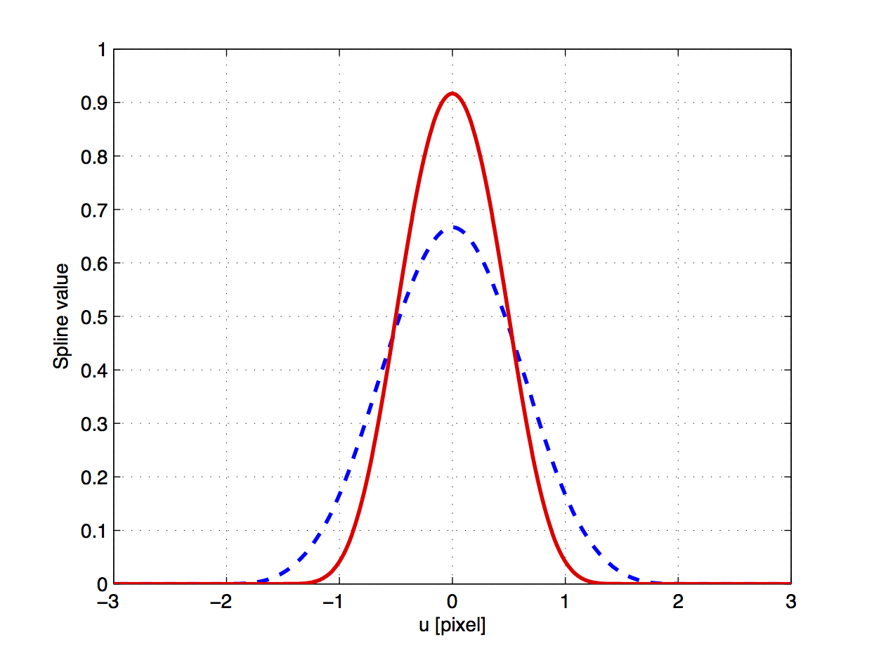
The S-splines used to represent the cores of the basis functions , and hence of , were obtained with and . They are thus quartic splines defined of a regular knot sequence with knot separation , and can be written as a linear combination of the functions , where
| (3.4) |
for . Alternatively, can be obtained by adding two adjacent quartic B-splines. Figure 3.10 shows this function together with the cubic B-spline for knot interval . Although both functions satisfy Equation 3.3, the S-spline can clearly represent peaks of the LSF that are narrower than is possible with the B-spline. Other choices than and are possible but have not been tested.
While the decomposition of a given spline in terms of B-splines is always unique, the decomposition in terms of is not necessarily unique. This is not a problem as long as the coefficients of are not directly used to parametrise the LSF, but are only used to represent pre-defined basis functions such as . When fitting an S-spline to , the possible non-uniqueness of the coefficients can be handled by using the pseudo-inverse.