1.1 The Gaia mission 1.1.2 Mission history and science case 1.1.4 Concepts of the scanning law

1.1.3 The spacecraft

Author(s): Jos de Bruijne, Juanma Martín-Fleitas, Alcione Mora, Jordi Portell

Overview

The spacecraft consists of a payload module (PLM; Section 1.1.3) with the instrument and a service module (SVM; Section 1.1.3) with support functions. The prime contractor of Gaia is Airbus Defence and Space (DS), Toulouse, France (formerly known as Astrium). An overview of the spacecraft is provided in Gaia Collaboration et al. (2016b).

Payload module

The payload module houses the two telescopes and the focal-plane assembly (FPA; Section 1.1.3). In addition, the payload houses the focal-plane computers (the video-processing units, VPUs, running the video-processing algorithms, VPAs; Section 1.1.3), the detector electronics (PEMs, for proximity-electronics modules; Hambly et al. 2018b), an atomic master clock (CDU, for clock-distribution unit; Section 1.1.3), metrology systems (basic-angle monitor, BAM, and wave-front sensors, WFSs; Section 1.1.3 and Section 1.1.3), and the payload data-handling unit (PDHU; Section 1.1.3). An overview of the payload module can be found in de Bruijne et al. (2010a) and Gaia Collaboration et al. (2016b).

Telescopes

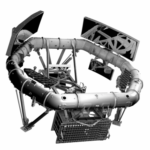
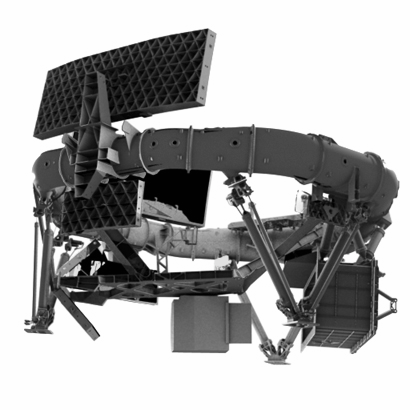
Gaia houses two ‘identical’ telescopes, sharing a common focal plane. The lines of sight of the telescopes are separated by a fixed angle called the basic angle ( $\Gamma=106{\hbox{$.\!\!^{\circ}$}}5$ ; see Lindegren et al. 2012, in particular their figure 2). Only when the basic angle is fixed, or when variations in it are known with high precision, can the stellar position (timing) measurements made in both lines of sight be connected and converted to angular separations on the sky (e.g., Butkevich et al. 2017). Both telescopes are three-mirror anastigmats (TMAs) with a Korsch off-axis configuration. The TMAs are of type concave-convex-concave and produce an intermediate image between the secondary and tertiary mirror. The entrance pupils are located at the rectangular primary mirrors, and have a dimension of $1.45\times 0.50$ m ${}^{2}$ . A beam combiner at the exit pupil merges the optical paths. Two further flat mirrors in the combined beam fold the light towards the focal plane. The total number of mirrors is hence 10 for both telescopes combined. The light path of the telescopes is illustrated in this video. The image quality of the telescope can be adjusted in flight through (five-degrees-of-freedom) mechanisms attached to the secondary mirrors. An overview of the payload and optical layout is displayed in Figure 1.1. More details on the telescopes are given in Gaia Collaboration et al. (2016b).

Figure 1.1: Schematic payload overview without protective tent. Most electronic boxes, e.g., clock distribution unit, video-processing units, or payload data-handling unit, are physically located in the service module and hence not visible here (see Figure 1.7). Figures from Gaia Collaboration et al. (2016b).

The focal length of both telescopes is 35 m, providing a plate scale of $58.9\times 176.8$ mas pixel ${}^{-1}$ in the along- (AL) and across-scan (AC) directions, respectively. Each telescope has a field of view of $1{\hbox{$.\!\!^{\circ}$}}8\times 0{\hbox{$.\!\!^{\circ}$}}7$ and achieves (near-)diffraction-limited image performance in the visible wavelength range (330-1050 nm).

The focal-plane assembly

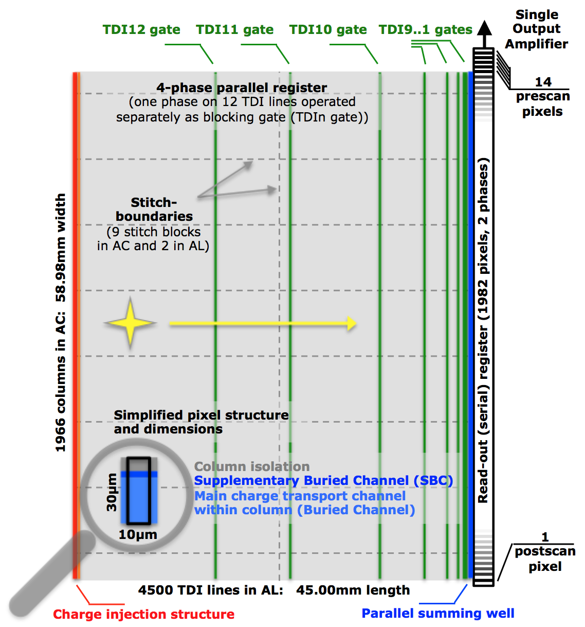
The focal-plane assembly (FPA) is shared by both telescopes. It houses 106 charge-coupled-device (CCD) detectors. Since Gaia is continuously scanning around its axis, the CCDs are operated in time-delayed integration (TDI) mode. Gaia’s measurements are very precise in the along-scan direction through precise timing of the signals (line-spread functions, LSFs; see Bastian and Biermann 2005 and Section 1.1.3). In the across-scan direction, the CCD images of most faint stars are binned, substantially reducing the CCD readout noise and science-data volume, with minimum impact on the astrometry. Details on Gaia’s operating principle are provided in Lindegren and Bastian (2010).

The focal plane houses five functionalities:

•

metrology (Section 1.1.3 and Section 1.1.3): a basic-angle monitor (BAM) composed of two detectors (one nominal and one redundant) continuously measures variations in the basic angle between the two telescopes. Two wave-front sensors (WFSs), with two associated detectors (one at the edge and one in the middle of the focal plane), allow monitoring the optical quality of the telescopes and support re-focusing (Section 1.3.3);
•

sky mapping (Section 1.1.3): both telescopes have their own sky-mapper (SM) detectors ( $7+7=14$ devices in total). These detectors allow detection of objects of interest (point sources as well as slightly extended sources such as asteroids and unresolved galaxies), identification of the parent field of view of each detection, and rejection of cosmic rays, Solar protons, etc.;
•

astrometry (Section 1.1.3): 62 CCDs are devoted to astrometry in the so-called astrometric field (AF);
•

spectro-photometry (Section 1.1.3): $7+7=14$ CCDs are devoted to low-resolution spectro-photometry in two different bandpasses. Spectra, dispersed along the scan direction, are generated through the use of a blue and a red prism (blue and red photometers, BP and RP);
•

spectroscopy (Section 1.1.3): 12 CCDs, arranged in three strips with four rows each, are devoted to spectroscopy. Medium-resolution spectra (resolving power $R\approx 11\,700$ , dispersed along the scan direction) are generated through an integral-field grating plate in the radial velocity spectrometer (RVS). The RVS instrument is described in detail in Cropper et al. (2018).

More details on the focal plane can be found in Gaia Collaboration et al. (2016b). The focal-plane layout is shown in Figure 1.2.

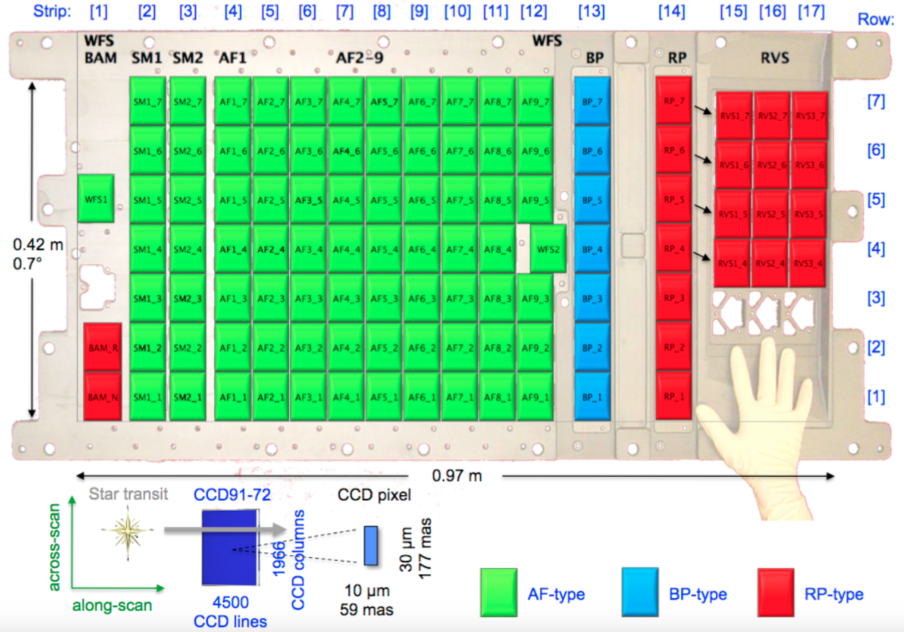
Figure 1.2: Schematic image of the focal-plane assembly, superimposed on a real picture of the CCD support structure (with a human hand to indicate the scale), with Gaia-specific terminology indicated: the focal plane consists of 17 strips and 7 rows with CCD detectors and each CCD has 4500 (TDI) lines along the scan direction and 1966 (pixel) columns across the scan direction. Figure from Gaia Collaboration et al. (2016b).

The 106 CCD detectors come in three different types: the broad-band CCD, the blue-enhanced CCD, and the red-enhanced CCD. Each of these types has the same architecture (e.g., number of pixels, TDI gates, readout register, etc.) but differ in their anti-reflection coating and surface passivation, their thickness, and the resistivity of their silicon wafer. The broad-band and blue CCDs are both 16 $\mu$ m thick and are both manufactured from standard-resistivity silicon; they differ only in their anti-reflection coating, which is optimised for short wavelengths for the blue CCD and optimised to cover a broad bandpass for the broad-band CCD. The red CCD, in contrast, is based on high-resistivity silicon, is 40 $\mu$ m thick, and has an anti-reflection coating optimised for long wavelengths. Quantum-efficiency considerations underly the choice of the detector variant for the various instruments: the broad-band CCD is used in the sky mapper (SM), in the astrometric field (AF), and for the wavefront sensor (WFS). The blue CCD is used in the blue photometer (BP). The red CCD is used in the basic-angle monitor (BAM), in the red photometer (RP), and in the radial velocity spectrometer (RVS).

Video-processing units and algorithms

The CCD detectors in the focal plane are commanded by video-processing units (VPUs). Gaia has seven identical VPUs, each one dealing with a dedicated row of CCDs (see Figure 1.2). Each CCD row contains, in order: two SM CCDs (one for each telescope), nine AF CCDs (except on row four, where the last detector is a wave-front sensor), one BP CCD, one RP CCD, and three RVS CCDs (the latter only for four of the seven CCD rows). The VPUs run seven identical instances of the video-processing algorithms (VPAs) albeit not necessarily with exactly the same parameter settings. This mix of some hardware and mostly software is responsible for object detection, detection confirmation, object windowing (see also Section 1.1.3), window-conflict resolution, data binning and prioritisation, science-packet generation, data compression, etc. More details on these functions can be found in Gaia Collaboration et al. (2016b) as well as in the below summary and in this video.

Object detection

The sky-mapper (SM) CCDs are systematically read in ‘full-frame’ mode albeit with on-chip (hardware) binning of $2\times 2$ pixels into a single sample. The object-detection chains for the first sky-mapper strip SM1 (imaging the preceding field-of-view) and the second sky-mapper strip SM2 (imaging the following field-of-view) are functionally identical, but their processing algorithms are parametrised independently to allow for, for instance, variations of the PSF over the focal plane. The detection algorithms scan the images coming from each SM in search for local flux maxima corresponding to celestial objects. A basic data treatment is applied before any on-board processing to correct the raw CCD sample data for gain and offset variations. For each local maximum detected after background removal, spatial-frequency filters in both the along- and the across-scan directions are applied to the flux distribution within a $3\times 3$ samples so-called working window that is centred on the local maximum. Objects failing to meet star-like PSF criteria are classified as prompt-particle event (PPE) or (bright-star) ripple, which means high-frequency or low-frequency outliers, respectively. More details can be found in de Bruijne et al. (2015).

Table 1.1: Definition of percentages of calibration faint stars (CFSs). These stars, which are used for several calibration and monitoring functions on ground, receive an ‘upgraded treatment’ on board and are assigned windows and sampling as if they were bright stars of sampling class 0 (see Table 1.2 and Figure 1.3). The percentage for the faintest magnitude bin (20.0–20.7 mag) was changed from 0% to 0.02% on 21 March 2017 (OBMT 4956.7) for VPU-5 and on 28 March 2017 (OBMT 4984.7) for the remaining VPUs. OBMT stands for on-board mission time(line) in units of six-hour revolutions since launch.

$G$ magnitude range	Percentage [%]
5.0–13.0	0.10
13.0–13.5	0.36
13.5–14.0	0.24
14.0–14.5	0.18
14.5–15.0	0.12
15.0–15.5	0.09
15.5–18.0	0.06
18.0–19.0	0.08
19.0–20.0	0.04
20.0–20.7	0.02

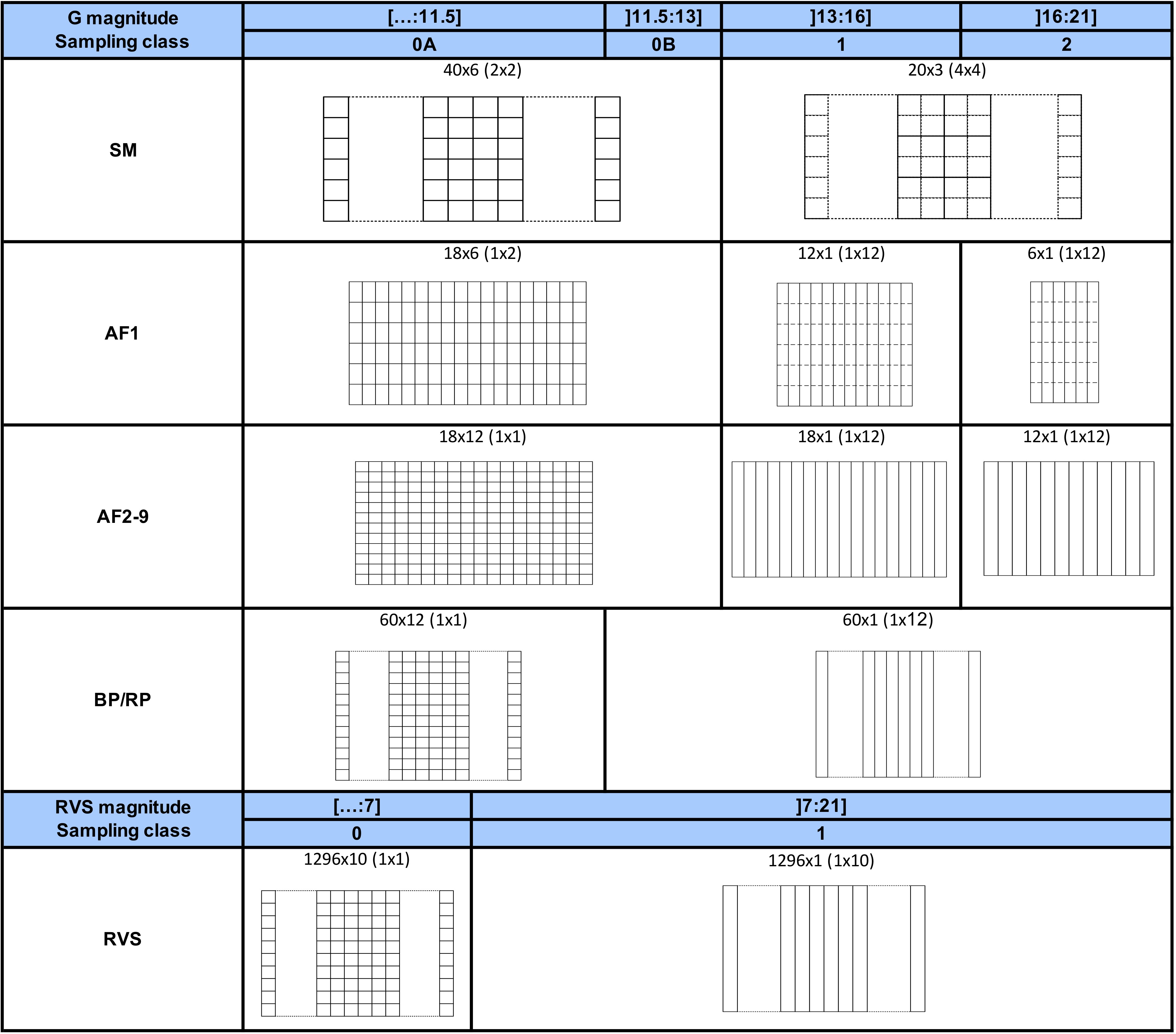
The surviving, star-like detections are classified either as faint detected object (non-saturated star) or saturated extremity (bright, saturated star). Detections are sorted by flux from high to low (bright to faint) and, subsequently, only up to a maximum of five objects per TDI line and field-of-view are retained for further processing in view of memory-sizing constraints. A list of detected objects is then produced with their attributes, mainly magnitude (computed from the flux, as explained below), observation priority (linked to magnitude), class of sampling (Table 1.2 and Figure 1.3), type, and along- and across-scan position. Saturated extremities of bright-star leading and trailing wings are matched on-board to produce bright-star detections. Next, a small, randomly-selected fraction of faint stars (Table 1.1) are upgraded to so-called calibration faint stars (CFSs), meaning that, rather than having one-dimensional windows as a result of across-scan binning, their windows are kept fully two-dimensional (as for bright stars); these data are used in the ground processing, for instance to monitor and calibrate the PSF as well as CCD cosmetic effects (Section 1.3.4). Finally, user-controlled virtual objects (VOs) are ‘artificially’ added to the list of detected objects. Since VOs are propagated across the various CCD detectors in the row controlled by each VPU, they normally result in empty (sky) windows readout from each device. VOs are therefore useful for various calibration purposes (e.g., Section 1.3.4 and Section 1.3.4).

Table 1.2: Definition of sampling classes – also called window classes – in the VPU. A graphical version can be found in Figure 1.3. Magnitude refers to

G

for SM, AF, and BP/RP and to

G_{\rm RVS}

for RVS. The window sizes refer to the data contained in the star packets that are transmitted to ground (Section 1.1.3). The sky-mapper (SM) bright detection limit is somewhere in the range

G

\sim 2

–3 mag but the on-board magnitude assignment of such bright stars saturates at

G

=5

mag. There is no direct, controlled RVS bright limit, i.e., there is no active rejection of too bright stars: the only requirement for a bright star to enter RVS, is to get detected in SM. The SM CCDs are read in ‘full-frame’ mode, in continuous search for celestial objects, but only small windows around confirmed detections are transmitted to ground. The indicated faint limits (21 mag) apply to the on-board magnitude coding (16 magnitudes, from

G_{\rm VPU}=5.016

to 21 mag, on 10 bits, so 1024 values). The true limits of the survey are defined by user-configurable flux thresholds, corresponding to

G

=20.7

mag for astrometry / photometry and to

G_{\rm RVS}

=16.2

mag for spectroscopy (see Section 1.3.3). The RVS along-scan window size was increased from 1260 to 1296 pixels in late April 2015, when the VPU application software was upgraded from version 2.7 to 2.8 (see Section 1.3.3).

Instrument	Sampling	Bright mag-	Faint mag-	Window size	Sample size
	class	nitude limit	nitude limit	(AL $\times$ AC samples)	(AL $\times$ AC pixels)
SM	0	5.0	13.0	$40\times 6$	$2\times 2$
SM	1	13.0	16.0	$20\times 3$	$4\times 4$
SM	2	16.0	21.0	$20\times 3$	$4\times 4$
AF1	0	5.0	13.0	$18\times 6$	$1\times 2$
AF1	1	13.0	16.0	$12\times 1$	$1\times 12$
AF1	2	16.0	21.0	$6\times 1$	$1\times 12$
AF2–9	0	5.0	13.0	$18\times 12$	$1\times 1$
AF2–9	1	13.0	16.0	$18\times 1$	$1\times 12$
AF2–9	2	16.0	21.0	$12\times 1$	$1\times 12$
BP/RP	0A	5.0	11.5	$60\times 12$	$1\times 1$
BP/RP	0B	11.5	13.0	$60\times 1$	$1\times 12$
BP/RP	1	13.0	16.0	$60\times 1$	$1\times 12$
BP/RP	2	16.0	21.0	$60\times 1$	$1\times 12$
RVS	0	N/A	7.0	$1296\times 10$	$1\times 1$
RVS	1	7.0	21.0	$1296\times 1$	$1\times 10$

Figure 1.3: Definition of sampling classes – also called window classes – in the VPU. A tabular version can be found in Table 1.2. Magnitude refers to $G$ for SM, AF, and BP/RP and to $G_{\rm RVS}$ for RVS. The window sizes refer to the data contained in the star packets that are transmitted to ground (Section 1.1.3). The notation ‘A $\times$ B (c $\times$ d)’ means A along-scan $\times$ B across-samples with each sample composed of c along-scan $\times$ d across-scan pixels. Dotted lines indicate numerical (software) binning of acquired samples on board before transmission to ground. Sampling class 0A and 0B combined is equivalent to class 0. The SM CCDs are read in ‘full-frame’ mode, in continuous search for celestial objects, but only small windows around confirmed detections are transmitted to ground, as depicted here. The RVS along-scan window size was increased from 1260 to 1296 pixels in late April 2015, when the VPU application software was upgraded from version 2.7 to 2.8 (see Section 1.3.3). Image based on a spreadsheet originally created by Airbus DS.

Detection confirmation

After sky-mapper (SM) detection, the available resources for observation in the AF instrument, which sees the light of both telescopes combined, are allocated to the list of SM-detected objects according to their priority (essentially magnitude). This allocation takes place after the first strip of the AF instrument (AF1; Figure 1.2) has been traversed and the associated data has been processed on board. Some SM-detected objects may be discarded at this stage due to a lack of resources (‘windows’; Section 1.1.3); this is especially true during Galactic-plane scans (GPSs; Section 1.1.5), i.e., periods of time during which the scanning law makes Gaia scan (roughly) along the Galactic plane for several consecutive days. Finally, a filtering stage using the AF1 data either confirms objects for observation or discards them in case no corresponding signal is observed in AF1 at the predicted location and moment in time.

On-board estimated magnitude

For each local maximum that passes the spatial-frequency filters in both the along- and the across-scan directions (see de Bruijne et al. 2015), a coarse estimate of the magnitude is made on board using the SM data for the purpose of activating TDI gates, selecting the appropriate windowing and sampling configuration, defining an observation priority for resource assignment and conflict resolution, deciding whether an object is suitable to contribute rate data in the closed-loop attitude control, and setting the priority level of the star packet in the payload data handling unit. As mentioned above, prior to any on-board processing, a basic treatment of the raw SM detector samples is applied to correct for gain and offset variations. The flux of the detected source is estimated as the sum of the counts of the 9 samples that compose the $3\times 3$ working window that is centred on each local maximum, after subtraction of an estimate of the local background flux per sample. The local background flux per sample is estimated as the fifth entry of the ranked list of the fluxes of the 16 samples in the background ‘ring’ that surrounds the $3\times 3$ working window (ranked means sorted from low to high fluxes). If the resulting, background-subtracted flux is negative, then it is set to zero. For stars without saturated samples in the SM data, an on-board magnitude estimate, denoted ${\rm g\_mag}$ , is computed as ${\rm round}(-263+69.5\cdot\log({\rm flux}))$ , where log is the natural logarithm. The relationship between ${\rm g\_mag}$ and $G_{\rm VPU}$ , which can be considered to be a proxy of the $G$ magnitude, is given by $G_{\rm VPU}=21-{\rm g\_mag}/64$ . This quantity is coded on 10 bits (1024 values) and covers a dynamic range of 16 mag ranging from 5.016 to 21 mag. The typical precision of magnitudes estimated in this way is a few tenths of a magnitude, with outliers appearing for a variety of reasons (background subtraction errors, flux contamination from nearby sources, etc.). Furthermore, for most stars fainter than 13 mag, the on-board estimated g_mag is refined on board after the AF1 CCD sample data has been collected. Using a similar processing as for the SM data, using a working window and a background ‘ring’ around the confirmed object, a background-subtracted AF1 flux is computed on board, after which an updated flux is computed as a weighted average of the SM flux and the AF1 flux ( ${\rm flux}=(128\cdot{\rm sm\_flux}+83\cdot{\rm af1\_flux})/256$ , where the ratio $83/128$ follows from the ratio of the integration times of SM and AF1, $2900/4494$ TDI lines), followed by an update of the on-board magnitude estimate. For bright stars that generate one or more saturated samples on board (typically $G_{\rm VPU}<13$ mag), a special branch exists in the on-board computations, in which the magnitude is estimated with use of a look-up-table that defines the relation between the size of the saturated area and magnitude based on a PSF model. Bright-star magnitude estimates are less precise than faint-star values and typical precisions are $\sim$ 1 mag. Although stars with magnitudes as bright as $G\sim 2$ mag and fainter than 21 mag are occasionally observed in SM as a result of the on-board magnitude estimation errors, the on-board magnitude assignment ‘saturates’ at $G_{\rm VPU}=5.016$ mag at the bright end and 21 mag at the faint end.

Bright-star handling

Stars brighter than $\sim$ 2–3 mag in the Gaia $G$ band are not properly detected on-board at each transit (e.g., Sahlmann et al. 2016). Special sky-mapper (SM) SIF images (see below) are therefore acquired for all of them in the sky-mapper CCDs. See Gaia Collaboration et al. (2016b) for details. These special SIF data are not part of Gaia EDR3.

Astrometric and photometric data

Only confirmed objects with AF1 data are observed in the full AF instrument (AF2–AF9). The observation windows, which are assigned according to the object’s sampling class (Table 1.2 and Figure 1.3), are centred on the expected object position on each CCD strip, following the along- and across-scan propagation determined from the attitude and orbit control sub-system, and have an initial rectangular shape. The final window shape and sample size per object is impacted by sample truncation, which can happen for a variety of reasons, including conflict management among partially-overlapping windows from different objects and windows crossing CCD boundaries in the across-scan direction.

As the objects reach the end of the AF instrument, similar algorithms as the ones described for AF are triggered for BP/RP. A new resource-allocation process is carried out, for BP and RP independently, optimising the observations based on the object priority while ensuring a constant number of samples per TDI line. The observation windows, which are assigned according to the sampling class of the object (Table 1.2 and Figure 1.3), are centred on the expected object position. As for AF, the final BP/RP window shape and sample size per object is impacted by sample truncation, which can happen for a variety of reasons, including conflict management among partially-overlapping windows from different objects and windows crossing CCD boundaries in the across-scan direction.

In order to limit VPU-memory usage and real-time VPU computations induced by the relatively long BP/RP windows (60 compared to 18 along-scan samples for AF), along-scan samples are not treated in isolation but in small groups referred to as ‘macro-samples’. Windows in BP/RP cannot start at arbitrary moments in the TDI stream but are all phased at macro-sample level. For instance resource-allocation and conflict-management computations on board are only performed for macro-samples, implying that any truncation of samples is identical within a given macro-sample. For BP/RP, the macro-sample size is 4 along-scan samples (TDI periods), such that 60-pixel windows should be thought of as being composed of 15 macro-samples, each covering 4 samples (pixels) along scan. Macro-samples are only a VPU-internal concept introduced to limit the processing load and do not impact the intrinsic (spectral) resolution of the data.

Table 1.3: TDI-gate characteristics.

$g$	SM	AF	BP/RP	RVS	TDI lines used	Exposure time	Exposure mid-time offset
						[TDI lines]	[TDI lines]
0		✓	✓	✓	3,4,7,8,11:4500	4494	2253.497330
1					3,4	2	3.500000
2					3,4,7,8	4	5.500000
3					3,4,7,8,11:14	8	9.000000
4		✓			3,4,7,8,11:22	16	13.750000
5			✓		3,4,7,8,11:38	32	22.125000
6					3,4,7,8,11:70	64	38.312500
7		✓	✓		3,4,7,8,11:134	128	70.406250
8		✓			3,4,7,8,11:262	256	134.453125
9		✓	✓		3,4,7,8,11:518	512	262.476562
10		✓			3,4,7,8,11:1030	1024	518.488281
11		✓	✓		3,4,7,8,11:2054	2048	1030.494141
12	✓	✓			3,4,7,8,11:2906	2900	1456.495862

Notes. Column 1 denotes the gate index

g

which is 0 for un-gated observations and 1–12 for gated observations (see main text for details), with

g=1

used for the brightest stars. The columns headed SM, AF, BP/RP, and RVS indicate which gates are in use in which part of the focal plane. The next column lists the TDI lines used for a given gate, with the TDI lines numbered from 1 to 4500, counted from the serial (readout) register (Figure 1.4). Note that TDI lines 1, 2, 5, 6, 9, and 10 are permanently blocked by a shield on top of the CCD such that they are not sensitive to light. The exposure time, measured in TDI-line periods of exactly 0.9828 ms of on-board time, is the total number of active (i.e., charge-collecting) TDI lines when a given gate is activated (or if none are activated when

g=0

). The notation 11:4500 means TDI lines 11 through 4500 (inclusive). The exposure mid-time offset is the mean value of the active TDI line numbers, and corresponds to the nominal location of the observation line (i.e., excluding centroid shifts induced by photo-response non-uniformities), expressed as the number of TDI periods before the instant when the pixel content is in the serial register.

When gathering the raw samples, the VPU temporarily limits the exposure time for bright stars as needed by activating user-defined TDI gates, both in the AF and in the BP/RP CCDs (Figure 1.4 and Table 1.3). SM CCDs are operated with TDI gate number $g=12$ permanently active to avoid excessive saturation of bright stars. Finally, in order to minimise the effect of charge-transfer inefficiency (CTI) due to native and radiation-induced charge trapping, a periodic charge injection (CI) is activated in each AF and BP/RP CCD (Section 1.3.4). This injection keeps slow traps permanently filled and, through periodically resetting the illumination history of the CCD, reduces the variance in the location bias that is induced by the celestial star pattern passing by a TDI line as Gaia scans the heavens (e.g., Short et al. 2013).

After the SM, AF, and BP/RP samples for an object have been collected, they are grouped to form a star packet of type 1 (SP1; Section 1.1.3) which is stored in the payload data-handling unit (PDHU; Section 1.1.3). The shape of the various windows is recorded in the SP1-packet header in order to facilitate the window-reconstruction process on-ground (Section 3.4.3; see also Section 3.1 in Fabricius et al. 2016). Each SP1 packet is time stamped with the object acquisition time in AF1. The packet is assigned a File_ID for (prioritised) on-board storage in the PDHU and for down-link prioritisation (Section 1.3.3).

Coincident with the generation of an SP1 packet, each observation is also entered into a so-called object log (ASD7; see Section 1.1.3), which is used on-ground for the detailed reconstruction of the readout process also in cases where not all star packets reach ground.

Figure 1.4: Gaia CCD detector layout. Stars move from left to right in the along-scan direction (yellow arrow). Charges in the readout register are clocked from bottom to top. The first line of the CCD (left) contains the charge-injection structure (red). The last line of the CCD before the readout register (right) contains the summing well and transfer gate (blue). Dashed, grey lines indicate stitch-block boundaries. Solid, green vertical lines indicate TDI gates (the three longest gates are labelled at the top of the CCD; Table 1.3). The inset shows some details of an individual pixel. Figure from Gaia Collaboration et al. (2016b).

Spectroscopic data

With part of the flux collected from the RP spectrum, an estimate of the magnitude of the object in the RVS instrument is produced before the object enters the RVS field. When this is not possible, the RVS magnitude is computed as an extrapolation from the AF magnitude. The object observation priority and class of sampling in RVS (Table 1.2 and Figure 1.3) is derived from this magnitude. Another separate resource-allocation process is carried out for the RVS. The observation windows, which are assigned according to the sampling class of the object (Table 1.2 and Figure 1.3), are centred on the expected object position. As for AF and BP/RP, the final RVS window shape and sample size per object is impacted by sample truncation, which can happen for a variety of reasons, including conflict management among partially-overlapping windows from different objects (see Cropper et al. 2018) and windows crossing CCD boundaries in the across-scan direction.

As for BP/RP, RVS processing loads on board are limited by the use of macro-samples. For RVS, the macro-sample size is 108 along-scan samples (TDI periods), such that 1296-pixel windows should be thought of as being composed of 12 macro-samples, each covering 108 samples (pixels) along scan. We stress, again, that macro-samples are only a VPU-internal concept introduced to limit the processing load and do not impact the intrinsic (spectral) resolution of the data.

After the RVS raw samples have been collected for an object, they are grouped to form a star packet of type 2 (SP2; Section 1.1.3) and stored in the PDHU. In RVS CCDs, charge injections and TDI gates are not applied (see Cropper et al. 2018 for details). The shape of the RVS windows is recorded in the header of the SP2 packet. Each SP2 packet is time stamped with the object acquisition time in AF1 and the packet is assigned a File_ID for PDHU storage and down-link prioritisation (Section 1.3.3).

Coincident with the generation of an SP2 packet, each observation is also entered into a so-called object log (ASD7; see Section 1.1.3), which is used on-ground for the detailed reconstruction of the readout process also in cases where not all star packets reach ground.

Service-Interface Function

The service-interface function (SIF) is a protocol to perform low-level communications with the Gaia payload, in particular the VPUs. It is extremely flexible and hence can have many functionalities. The SIF function is able to read portions (take snapshots) of the VPU random-access memory, while the VPU is nominally operating, and store them in SIF data packets, which are subsequently down-linked to ground. Since the SIF function is versatile and non-invasive, it is not only useful as engineering tool to diagnose and solve problems affecting the VPU, it can also be used to add extra functionality that is not included in the VPU software. The SIF function is frequently used on Gaia, both to provide dumps of VPU-parameter memory blocks in order to validate the (tracking of the) configuration state of the VPU/VPA parameters in the configuration database (CDB; Section 1.2.3 and Section 1.3.3) and to acquire data that come directly from the detector electronics (the proximity-electronics modules, PEMs) and that are temporarily stored in the VPU memory before a fraction of the relevant information is extracted for inclusion in star packets. In this way, the SIF function allows extracting data that is not available in the nominal telemetry, for instance post-scan pixels to monitor radiation damage in the serial (readout) register (Section 1.3.4) or full-frame sky-mapper (SM) images to map selected dense areas (see next).

Dense-area handling

Gaia cannot cope with extremely dense areas on the sky. As explained in Gaia Collaboration et al. (2016b), the crowding limit is a few $100\,000$ objects per square degree for astrometry and photometry; for spectroscopy, the limit is around $35\,000$ objects per square degree. For a handful of selected, dense areas (Table 1.4), special SIF images (see above) are acquired in the sky-mapper (SM) CCDs to support the management of overlapping windows (deblending of images) in the ground processing. More details are provided in Gaia Collaboration et al. (2016b). These special SIF data are not part of Gaia EDR3.

Table 1.4: Selected dense areas in which special sky-mapper (SM) SIF images are collected, together with the start date of these acquisitions. SIF images have been acquired during most transits of these regions as of this start date. Before 1 January 2015, both the Sgr I and Baade’s bulge windows were observed once (both on 15 October 2014).

Name	Start date
$\omega$ Cen = NGC 5139	01-01-2015
Baade’s bulge window	01-01-2015
Sgr I bulge window	01-07-2016
Small Magellanic Cloud (SMC)	01-07-2016
Large Magellanic Cloud (LMC)	01-07-2016
M22 = NGC 6656	01-07-2016
M4 = NGC 6121	01-07-2016
47 Tuc = NGC 104	01-07-2016
NGC 4372	01-07-2016

Payload data-handling unit

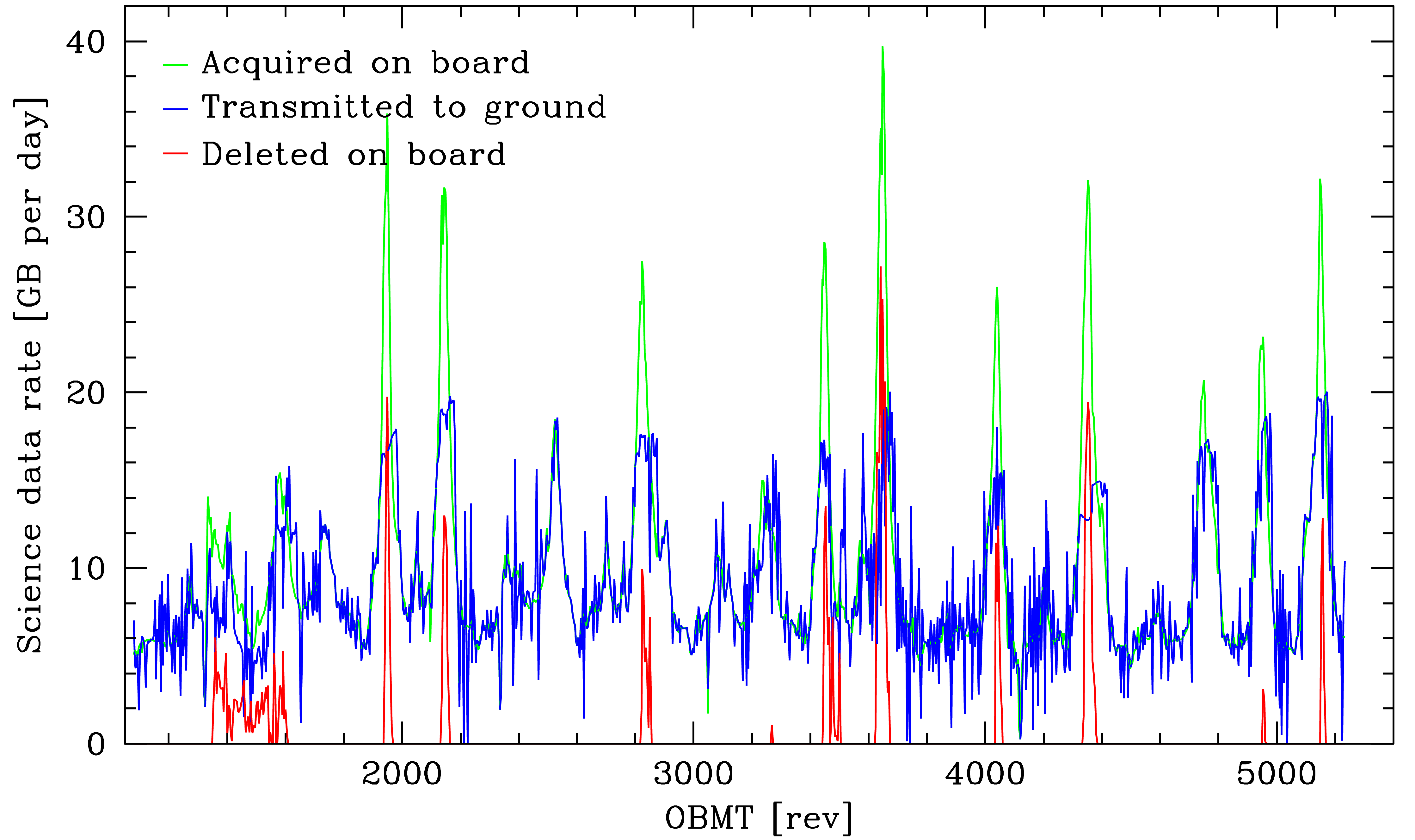
Star packets with science data that are generated on board in the VPUs (Section 1.1.3) are stored in the payload data-handling unit (PDHU) before being down-linked to ground. In order to support user-defined prioritisation of the science telemetry, the PDHU can handle up to 256 different files to store data, each labelled with a unique File_ID. The VPUs assign File_IDs to each star packet generated on board, partially based on user-defined settings. In general, bright stars have a higher down-link priority than faint stars. Under average sky conditions, the PDHU can contain several days worth of science data. However, when the scanning law makes Gaia scan (roughly) along the Galactic plane for several consecutive days (known as a Galactic-plane scan, GPS; Section 1.1.5), the PDHU saturates and a user-defined prioritisation scheme comes into play to govern on-board data deletion (see also Section 1.3.3). This happens a few times per year (Figure 1.5). In general, bright stars have a higher deletion protection than faint stars. More details on the PDHU are provided in Gaia Collaboration et al. (2016b).

Figure 1.5: Evolution of the science data rate over the time interval underlying Gaia EDR3. Shown are the daily rates at which the payload data-handling unit (PDHU) accumulates (green), deletes (red), and transmits (blue) science data. These data are losslessly compressed by a factor $\sim$ 2.5. Deletion of (low-priority) science data results primarily from the interplay of the scanning law with the Galactic plane, where the red peaks align with the galactic-plane scans (GPSs; Section 1.1.5).

Clock distribution unit

The clocking of all CCD detectors as well as the time tagging of the science data is based on a high-accuracy atomic rubidium clock, embedded in the clock distribution unit (CDU). The CDU contains a rubidium atomic frequency standard (RAFS). This clock is stable to within a few ns over a six-hour spacecraft revolution and has very small temperature, magnetic field, and input voltage sensitivities. The free running on-board time (OBT) counter, which is the time tag of all science data, is generated from the master clock. The spacecraft-elapsed time (SCET) counter in the central data management unit (CDMU), which is used for time tagging housekeeping data and for spacecraft operations, is continuously synchronised to OBT using a pulse-per-second (PPS) mechanism. More details on the CDU are contained in Gaia Collaboration et al. (2016b).

Wave-front sensor

Since telescope alignment has been performed on ground, it has been significantly influenced by gravitational forces acting on the payload. Although such forces were considered during the alignment, a non-negligible residual mis-alignment was expected in orbit. Hence, in order to achieve the required optical performance in flight, two CCDs in the focal plane are equipped with wave-front sensors (WFSs) to enable monitoring the optical quality of the telescopes through the observation of bright stars (Figure 1.2). The WFSs also allow deriving information to actuate the M2 mirror mechanisms to (re-)align and (re-)focus the telescopes in orbit (Section 1.3.3). These mechanisms contain high-precision actuators that can move the secondary mirrors of both telescopes in all five, relevant degrees of freedom, with only a rotation around the optical axis not supported.

The WFSs are of Shack-Hartmann type and contain an optical mirror that images both telescope entrance pupils on a dedicated CCD sensor in the focal plane. Each telescope pupil image is sampled with an array of $3\times 9$ micro-lenses. The latter focus the light of bright stars transiting the focal plane on the WFS CCDs. Comparison of the stellar spot pattern with the pattern of a built-in calibration source (used during initial tests after launch) and with the ‘ideal’ pattern of stars acquired after achieving best focus (used afterwards during scientific operations; Section 1.3.3) allows reconstruction of the wave-front. See Gaia Collaboration et al. (2016b) for details.

Basic-angle monitor

The Gaia measurement principle relies on the ability to convert differences in the transit times between stars observed by each telescope into their angular separation on the sky (Lindegren and Bastian 2010; Gaia Collaboration et al. 2016b). The fundamental pre-requisite in this process is that the basic angle, i.e., the angle between the two telescopes (Section 1.1.3), either is ultra-stable or that its variations are known to better than $\sim$ 1 $\mu$ as. Two CCDs in the focal plane are part of the basic-angle monitor (BAM; Figure 1.2). The BAM allows monitoring variations of the basic angle of the telescopes (see Section 1.3.3) to $\mu$ as-levels every 15 minutes or shorter:

•

Low-frequency variations of the basic angle ( $f<1/2P_{\rm rot}$ , with $P_{\rm rot}=6$ h denoting the Gaia rotation period) can be fully eliminated by self-calibration (Lindegren and Bastian 2010), that is long-period basic-angle variations can be estimated from the science data themselves in the astrometric processing;
•

High-frequency, random variations are also not a concern because they are averaged out during all transits;
•

Intermediate-frequency variations, however, are difficult to eliminate by self-calibration and are therefore monitored by the BAM. Such basic-angle variations are even fundamentally impossible to calibrate, and can lead to a global, systematic error in the parallax zero point, if they are synchronised with the spacecraft spin phase (Butkevich et al. 2017).

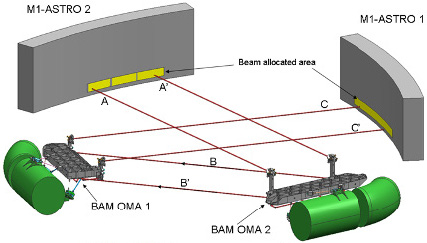
The BAM device is continuously measuring differential changes in the basic angle. It generates one fixed, artificial star per telescope by introducing two collimated laser beams into each primary mirror (see Figure 1.6). The BAM is composed of two optical benches in charge of producing the interference pattern for each telescope. A number of optical fibres, polarisers, beam splitters, and mirrors are used to generate all four beams from one common light source (see Gielesen et al. 2012). Each Gaia telescope then generates an image on the same, dedicated BAM CCD, which is an interference pattern due to the coherent input light source. The relative displacement between the two fringe patterns is a direct measurement of the basic-angle variations.

Figure 1.6: The BAM is a laser interferometer that injects two light beams in each telescope entrance pupil. In this way, an interference pattern is produced for each telescope in the common focal plane. The relative shift of the patterns at the level of the CCD is directly related to changes in the basic angle between the telescopes. Figure from Fabricius et al. (2016).

A detailed description of the BAM data collection and daily processing is provided in Section 7 of Fabricius et al. (2016).

Astrometric instrument

The astrometric field (AF) contains 62 CCDs in nine strips and seven rows, minus one CCD for the WFS in focal-plane strip 12 (AF strip 9) and row four (Section 1.1.3; Figure 1.2). The bandpass of the AF detectors, defining the Gaia $G$ band, covers 330–1050 nm; this is mainly set by the telescope transmission in the blue (resulting from the protected-silver coating on the mirrors) and the CCD response at long wavelengths. The AF CCDs are not read out in full but only small ‘windows’ around objects of interest are read out (Table 1.2 and Figure 1.3; see also Section 1.1.3). The typical window for faint stars is $12\times 12$ pixels (along-scan $\times$ across-scan), with the 12 pixels in the across-scan direction binned on chip into one single number (the intensity of the along-scan line-spread function, LSF). For bright stars ( $G$ $<13$ mag), single-pixel-resolution windows are used, of size $18\times 12$ pixels (along-scan $\times$ across-scan; Table 1.2 and Figure 1.3). For more details on the astrometric instrument, see Gaia Collaboration et al. (2016b).

Photometric instrument

The photometric instrument consists of two fused-silica prisms, known as the blue photometer (BP, covering 330–680 nm) and the red photometer (RP, covering 630–1050 nm). Both prisms are mounted inside the focal-plane assembly. Each prism has a selective bandpass filter that is implemented through multi-layer coatings. The two prisms form low-dispersion spectra in the along-scan direction. The spectral dispersion of the photometric instrument is a function of wavelength and varies in BP from 3 to 27 nm pixel ${}^{-1}$ over the wavelength range 330–680 nm. In RP, the spectral dispersion varies from 7 to 15 nm pixel ${}^{-1}$ over the wavelength range 630–1050 nm. The photometric instrument contains two CCD strips – one for BP and one for RP – and seven CCD rows (Figure 1.2). Object windows measure $60\times 12$ pixels (along-scan $\times$ across-scan; Table 1.2 and Figure 1.3; see also Section 1.1.3). Except for bright stars ( $G$ $<11.5$ mag), for which single-pixel-resolution windows are used, the 12 pixels in the across-scan direction are binned on chip into one single number. For more details on the photometric instrument, see Gaia Collaboration et al. (2016b) and Riello et al. (2018).

Spectroscopic instrument

The main aim of the spectroscopic instrument, already revealed by its common name, the radial velocity spectrometer (RVS), is to measure the radial velocity of the brightest subset of Gaia targets through Doppler shifts of absorption lines in the spectral range 845–872 nm, which covers the CaII triplet. The optical design of the RVS, which has a nominal resolving power of $11\,500$ , consists of a bandpass-filter plate, a number of fused-silica prisms, and an integral-field transmission grating. Two of the four prisms are of Féry type, having curved optical surfaces. The spectrometer optics are installed between the last folding mirror of the telescope and the focal plane. The spectroscopic instrument contains 12 CCDs, arranged in three strips and four rows (Figure 1.2). Dispersion of light takes place in the along-scan direction and windows measure $1296\times 10$ pixels (along-scan $\times$ across-scan; Table 1.2 and Figure 1.3; see also Section 1.1.3). Except for bright stars ( $G_{\rm RVS}$ $<7$ mag), for which single-pixel-resolution windows are used, the 10 pixels in the across-scan direction are binned on chip into one single number. For more details on the spectroscopic instrument, see Gaia Collaboration et al. (2016b) and Cropper et al. (2018).

The raw science telemetry data

The raw science data generated on-board by the video-processing units (VPUs; Section 1.1.3) consists of star packets (SPs) and auxiliary science data (ASD) packets. The former contain the science data itself, i.e., the pixel and sample readings acquired from the CCD detectors. The latter contain ‘shared data’, such as information on the measurement coordinates through the focal plane and the integration time of each image, that are needed for the reconstruction of measurements.

There are nine types of star packets, denoted SP1 to SP9, plus seven types of auxiliary science data packets, denoted ASD1 to ASD7. In addition, there are service-interface-function (SIF) packets that are mainly used for payload diagnostics and extended, on-demand data acquisitions (Section 1.1.3). SIF data do not enter the regular data-processing pipelines and have been treated separately for Gaia EDR3.

Star packets are not self-contained: in order to extract the relevant astrometric, photometric, and spectroscopic information for a given star, several star packets and auxiliary science data packets need to be combined. This reconstruction of individual measurements is performed as part of the astrometric and photometric pre-processing (Chapter 3) through a process called initial data treatment (IDT; Section 3.4.2).

Packet generation

Star Packets are generated as follows, where a source transit across (a part of) the Gaia focal plane refers to a VPU detection, confirmation, and measurement of the transit of an astronomical source (the contents of the various packets are summarised below this listing):

•
Nominal astronomical packets:
- –
  
  SP1 packets, which are the most abundant type, with one packet generated for each astronomical source transit across the SM, AF, and BP/RP CCDs. These packets form the main data input to all Gaia data processing systems.
- –
  
  SP2 packets come in addition to SP1 but only for those sources detected in the focal plane rows that have RVS CCDs (Figure 1.2) and only for those sources which are bright enough for being measured there.
- –
  
  SP3 packets are generated only in conjunction with SP1 packets for objects for which a significant across-scan motion has been autonomously detected on board. Such sources, typically Solar-system objects, are called suspected moving objects (SMOs).
•
Nominal instrumental packets:
- –
  
  SP4 packets, with regular (periodic) measurements from the basic-angle monitoring (BAM) device (Section 1.1.3).
•
Non-nominal astronomical packets:
- –
  
  SP6 (‘zoom+gate’) and SP7 (‘gate’) packets, with SM and AF1 measurements of bright stars. These are only generated either when the on-board attitude and orbit control sub-system (AOCS; Section 1.1.3) is being initialised or when it temporarily loses ‘closed-loop convergence’. These packets are generated and down-linked only for ground analysis and checks and do not enter the main data-processing pipelines.
- –
  
  SP8 (‘AF1 snapshot’) and SP9 (‘SM full readout’) packets, with AF1 or SM measurements of bright stars, which are also only generated under non-nominal on-board attitude-control situations. Also these packets do not enter the main data-processing pipelines.
•
Non-nominal instrumental packets:
- –
  
  SP5, with measurements from the wave-front sensors (WFSs; Section 1.1.3).

Auxiliary Science Data packets are generated as follows:

•

ASD1, with the across-scan window position information for all AF, BP/RP, and RVS CCDs, generated every second for each VPU.
•

ASD2, with electronic bias data (pre-scan pixels; Figure 1.4 and Section 1.3.4) of the detectors, generated about once per minute per VPU.
•

ASD3, with information on RVS spectral-resolution changes, generated every time that a bright star requiring high-resolution data is observed in an RVS CCD. As straylight mitigation measure (Section 1.3.3), it was decided early on in the mission to use always the high-resolution acquisition mode in RVS (Cropper et al. 2018). As a result, ASD3 packets are not available for most of the mission.
•

ASD4, with statistical information and counters related to processing events in the on-board detection chain, generated once every few seconds.
•

ASD5, with the times of activation of electronic charge injections (CI) in the CCDs, generated once every few seconds (Section 1.3.4).
•

ASD6, with the information on the TDI-gate activations in the CCDs (Section 1.1.3 and Table 1.3). These packets are generated every time that a bright star ( $G$ $<12$ mag) is observed in a CCD in order to reduce their integration time and hence limit saturation.
•

ASD7, containing the positions of the AF1 windows and the magnitudes for each confirmed detection that has been acquired by any VPU regardless whether the generating SP packets survive on-board storage and/or reach the ground or not. ASD7 packets, also known as object logs, are generated for each source transit – although an ASD7 packet actually contains information on a set of transits – as crucial input for the non-uniformity calibration (Section 1.3.4 and Hambly et al. 2018b).

Packet contents

The following are the contents of each of the raw telemetry packets down-linked by Gaia to the ground stations (see also Table 1.2 and Figure 1.3 for a summary of the windowing and sampling scheme):

•
SP1: these are the most important data packets. One SP1 packet contains the SM, AF, BP, and RP samples from one source transit over the focal plane. Only small ‘windows’ of samples are acquired and transmitted, centred by the VPU algorithms on the astronomical source:
- –
  
  For SM, windows of $40\times 6$ samples (each $2\times 2$ pixels) are sent, thus covering an area of about $4.7\times 2.1$ arcsec ${}^{2}$ . For objects fainter than 13 mag the windows are transmitted as $20\times 3$ samples (each 4 $\times$ 4 pixels).
- –
  
  For AF CCDs, the exact shape of the windows depends on the CCD (AF1 to AF9) and on the source brightness, but typically windows of $12\times 12$ pixels are sent (with the AC pixels binned into one single sample, thus providing only 12 samples in the AL or scanning direction). Bright stars ( $G$ $<16$ mag) are acquired with larger windows ( $18\times 12$ pixels), with the brightest sources ( $G$ $<13$ mag) being acquired in full, two-dimensional resolution (without across-scan pixel binning). Thus, AF windows typically cover $0.7\times 2.1$ arcsec ${}^{2}$ on the sky (increasing to $1.0\times 2.1$ arcsec ${}^{2}$ for bright sources).
- –
  
  BP/RP windows cover $60\times 12$ pixels, with the 12 AC pixels normally binned into one single sample. Only for the brightest sources ( $G$ $<11.5$ mag), this binning is not applied resulting in windows with two-dimensional resolution.
- –
  
  Besides the raw CCD samples, SP1 packets also include the time, field of view, CCD row, and across-scan pixel coordinate where the source was detected (all based on and with respect to the AF1 CCD), an on-board estimated magnitude, and information about the exact sampling scheme used, including information on the window shape, as windows may be truncated due to overlaps with another, nearby source.
•

SP2: these packets, as SP1 packets, also include the basic detection and measurement information but the only CCD sample data included is from the RVS CCDs. Three windows are included, one for each of the three along-scan RVS CCDs in a spectroscopic transit, each covering an area of $1296\times 10$ pixels ( $76.4\times 1.8$ arcsec ${}^{2}$ on the sky). The 10 AC pixels are normally binned into one single sample. Only for the brightest stars ( $G_{\rm RVS}<7$ mag), this binning is not applied resulting in windows with two-dimensional resolution.
•

SP3: these packets are complementary to SP1 packets for suspected moving objects (i.e., objects for which the VPU has detected a significant, excess across-scan motion from SM to AF1). Here, only basic detection information is included (as in SP2), and the only CCD sample data is that from additional BP/RP windows placed above or below the nominal BP/RP windows, at the same along-scan coordinates, that are already included in the associated SP1 packet.
•

SP4: these packets include BAM CCD samples, with $500\times 80$ pixels centred on the on-board-configured BAM fringe centre, plus timing and position information of the BAM windows.
•

SP5: WFS data packets include windows of $682\times 120$ pixels plus timing and position information of the WFS windows.
•

SP6, SP7, SP8, and SP9 packets are non-nominal packets that are, for instance, generated during periods of non-nominal attitude control. They include, besides timing, position, and measurement information, windows of SM and AF1 samples (SP6 and SP7), AF1 samples (SP8), or SM samples (SP9). In these cases, the AF1 windows are much larger than the usual ones.
•

ASD1: each of these packets includes, besides a reference time and the CCD-row number, the across-scan shift in pixels with respect to the AF1 reference coordinate for each of the CCDs and for each field of view, expressed in pixels. Thus, only when combining the relevant ASD1 packet with an SP1 (or SP2 or SP3) packet, one can determine the absolute across-scan position where each window was acquired.
•

ASD2: each ASD2 packet contains a ‘burst’ of pre-scan samples acquired on a given CCD. These packets contain a CCD identifier, a reference time, and a set of typically 1024 CCD samples.
•

ASD3: these contain a reference time and CCD identifier, plus the RVS spectral-resolution switch type (low-to-high or high-to-low).
•

ASD4: there are two variants of these packets, both containing a large set of on-board counters (per VPU), such as the number of detected, confirmed, and allocated objects (that is, transits of astronomical sources) for the different types of windows and per field of view, or the number of packets generated of each SP/ASD type.
•

ASD5: each of these packets holds a set of time stamps (with respect to a packet reference time) when a charge injection was generated for a given CCD. One of these packets can cover between a few seconds up to $\sim$ 1–2 minutes of on-board time.
•

ASD6: each ASD6 packet indicates the TDI-gate configuration that was active for a given CCD at a given time. A new ASD6 packet is generated whenever the gate configuration changes, typically every time a TDI-gated window is started or finished.
•

ASD7: each ASD7 packet contains a reference time stamp plus a set of up to 3071 entries, each corresponding to one SP1 and SP2 packet allocated on board for the measurement of a source transit. Each such entry indicates the detection features (time, coordinate, field of view, acquisition mode, etc.) and the brightness of the source.

Besides the raw science data coming from the spacecraft, other ancillary data is also needed when performing the on-ground reconstruction of the raw measurements. Such data is stored in the so-called calibration database (CDB; Section 1.2.3), which contains the full history of the VPU configuration. An example of ancillary data needed are the along-scan phasing tables (ALPTs) from which, when combined with an AF1 detection time, the absolute measurement times for each of the windows in an SP1, SP2, or SP3 packet can be determined. Several other tables are also needed from the CDB, such as those that indicate the exact configuration for the TDI gates, charge injections, etc.

Service module

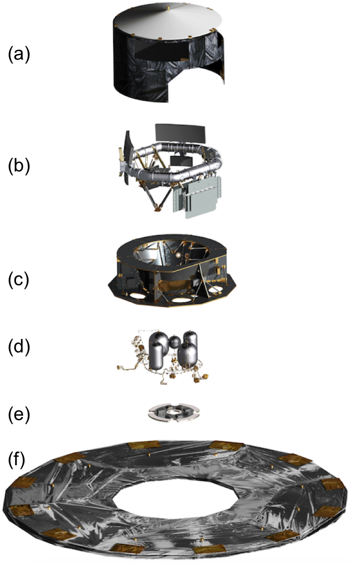
The service module (SVM) supports the payload, both mechanically / structurally and electronically / functionally. A description of the service module can be found in Gaia Collaboration et al. (2016b). The service module includes, for instance, the chemical and micro-propulsion sub-systems, the deployable-sunshield assembly, the payload thermal tent, the solar-array panels, and the electrical harness. Several electronic boxes, such as the video-processing units, payload data-handling unit, and clock distribution unit, functionally belong to the payload module but are housed in the service module in view of the required thermal stability of the payload. The electrical services of the service module support functions to the payload and spacecraft for attitude and orbit control, power control and distribution, central data management and software, thermal control and monitoring, and communications with the Earth. An exploded view of Gaia and the service module in particular, listing some major sub-systems, is shown in Figure 1.7.

The attitude and orbit control sub-system (AOCS) is based on a closed-loop design and relies on a star tracker for pointing and on payload data of bright, well-behaved stars for rate control. The alignment between the star tracker, which is physically located in the service module, and the focal plane in the payload module is regularly calibrated. In case of disturbances, such as micro-meteoroid impacts, the attitude and orbit control sub-system autonomously switches back and forth between three modes, which have different pointing and rate performance and which require different star packets from the payload (Section 1.1.3): converged, ‘normal (science) mode’ based on SP1 packets, ‘gate mode’ based on SP7 packets, and ‘zoom+gate mode’ based on SP6 packets. Further details on the scanning law that is materialised by the attitude and orbit control sub-system are described in Section 1.1.4 and Section 1.3.2.

Housekeeping and raw attitude data

The spacecraft generates a broad range of housekeeping parameters that are used for spacecraft health and safety monitoring at the Mission Operations Centre (Section 1.1.5). Included in the housekeeping data are raw attitude quaternions that are determined once per second by the attitude and orbit control sub-system (Section 1.1.3). These data are used by the Initial Data Treatment (Section 3.4.2) as a reference for the initial on-ground attitude determination and refinement (Section 3.4.5).

gaia early data release 3 documentation