3.4.13 Cross-match processing

The images detected on board, in the real-time analysis of the sky mapper data, are propagated to their expected transit positions in the first strip of astrometric CCDs, AF1, i.e., their transit time and AC column are extrapolated and expressed as a reference acquisition pixel. This pixel is the key to all further on-board operations and to the identification of the transit. For consistency, the cross-match does not use any image analysis other than the on-board detection, and is therefore based on the reference pixel of each detection, even if the actual image in AF1 may be slightly offset from it. This decision was made because, in general, we do not have the same high-resolution SM and AF1 images on ground as the ones used on board.

The first step of the cross-match is the determination of the sky coordinates of the Gaia detections, but only for those considered genuine. As mentioned, the sky coordinates are computed using the reference acquisition pixel in AF1. The precision is therefore limited by the pixel resolution as well as by the precision of the on-board image parameter determination. The conversion from the observed positions on the focal plane to celestial coordinates, e.g., right ascension and declination, involves several steps and reference systems, as shown in Figure 3.15.

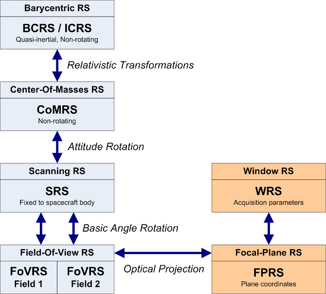
The reference system for the source catalogue is the Barycentric Celestial Reference System (BCRS/ICRS), which is a quasi-inertial, relativistic reference system that is non-rotating with respect to distant extra-galactic objects. Gaia observations are more naturally expressed in the Centre-of-Mass Reference System (CoMRS), which is defined from the BCRS by special relativistic coordinate transformations. This system moves with the Gaia spacecraft and is defined to be kinematically non-rotating with respect to the BCRS/ICRS. The BCRS is used to define the positions of the sources and to model the light propagation from the sources to Gaia. Observable proper directions towards the sources as seen by Gaia are then defined in the CoMRS. The computation of observable directions requires several pieces of additional data such as the Gaia orbit in the Solar system, a Solar system ephemerides, etc. As a next step, we introduce the Scanning Reference System (SRS), which is co-moving and co-rotating with the body of the Gaia spacecraft, and is used to define the satellite attitude. Celestial coordinates in the SRS differ from those in the CoMRS only by a spatial rotation given by the attitude quaternions. The attitude used to derive the sky coordinates for the daily system is the IDT OGA1 whereas the cyclic cross-match used the IDU SDMOGA reconstruction (similar to OGA1 in method and quality) both described in Section 3.4.5.

We now introduce separate reference systems for each telescope, called the Field-of-View Reference Systems (FoVRSs) with their origins at the centre of mass of the spacecraft and with the primary axis pointing to the optical centre of each of the fields, while the third axis coincides with the one of the SRS. Spherical coordinates in this reference system, the already mentioned field angles ($\eta ,\zeta$), are defined for convenience of the modelling of the observations and instruments. Celestial coordinates in each of the FoVRSs differ from those in the SRS only by a fixed nominal spatial rotation around the spacecraft rotation axis, namely by half the basic angle of $\mathrm{\Gamma }=106{.}^{\circ }5$ (Section 1.1.3).

Finally, and through the optical projections of each instrument, we reach the Focal Plane Reference System (FPRS), which is the natural system for expressing the location of each CCD and each pixel. It is also convenient to extend the FPRS to express the relevant parameters of each detection, specifically the field of view, CCD, TDI gate, and pixel. This is the Window Reference System (WRS). In practical applications, the relation between the WRS and the FoVRS must be modelled. This is done through a geometric calibration, expressed as corrections to nominal field angles as detailed in Section 4.3.6.

The geometric calibration used in the cross-match in the daily pipeline is derived by the First-Look system in the ‘One-Day Astrometric Solution’ (ODAS; Section 3.4.5) whereas the calibration used in the cyclic cross-match is the combination of ODAS solution for the more recent data segments and the ‘Astrometric Global Iterative Solution’ (AGIS; Section 4.4.2) for the rest.

The scene is in charge of providing a prediction of the objects scanned by the two fields of view of Gaia according to the spacecraft attitude and orbit, the planetary ephemerides, and the source catalogue. It was originally introduced to track the illumination history of the CCD columns for the parametrization of the CTI mitigation. However, this information is also relevant for:

• •

  The astrophysical background estimation and the LSF/PSF profile calibration, to identify nearby sources that may be affecting a given observation. The scene can easily reveal if the transit is disturbed or polluted by a parasitic source.

• •

  The cross-match, to identify sources that will probably not be detected directly, but still leave many spurious detections, for example from diffraction spikes or internal reflections.

Therefore, the scene does not only include the sources actually scanned by both fields of view but it also identifies:

• •

  Sources without the corresponding Gaia observations. This can happen in case of, e.g.:

  • –

    Very bright sources (brighter than $\sim 6^{\mathrm{th}}$ magnitude) or transits of solar-system objects (SSOs) that are not detected in the Sky Mapper (SM) or not confirmed in the first CCD of the Astrometric Field (AF1).

  • –

    Fast SSOs, detected in SM but not successfully confirmed in AF1.

  • –

    High-density regions in which the on-board resources (windows) are insufficient in number to cover all detected objects.

  • –

    Close neighbours on the sky for which the detection and acquisition of two separate observations is impossible (Section 1.1.3).

  • –

    Data losses due to on-board storage overflow, data transfer issues, or processing errors.

• •

  Sources falling into the edges and between CCD rows.

• •

  Sources falling out of both fields of view but so bright that they may disturb or pollute nearby observations.

It must be noted that the scene is established not from the individual observations, but from the catalogue sources and planetary ephemerides. The scene is therefore limited by the completeness and quality of those input tables.

The Gaia on-board detection software was built to detect point-like images on the SM CCDs and to autonomously discriminate star images from cosmic rays, etc. For this, parametrised criteria of the image shape are used, which need to be calibrated and tuned. There is clearly a trade-off between a high detection probability for stars at the faint end and keeping the detections from bright-star diffraction spikes (and other disturbances) at a minimum. A study of the detection capability, in particular for non-saturated stars, double stars, unresolved external galaxies, and asteroids is provided by de Bruijne et al. (2015).

The main problem with spurious detections arises from the fact that they are numerous (15–20% of all detections), and that each of them may lead to the creation of a (spurious) new source during the cross-match. Therefore, a classification of the detections as either genuine or spurious is needed to only consider the former in the cross-match.

As described in Torra et al. (2020), the main categories of spurious detections found in the data so far are:

• •

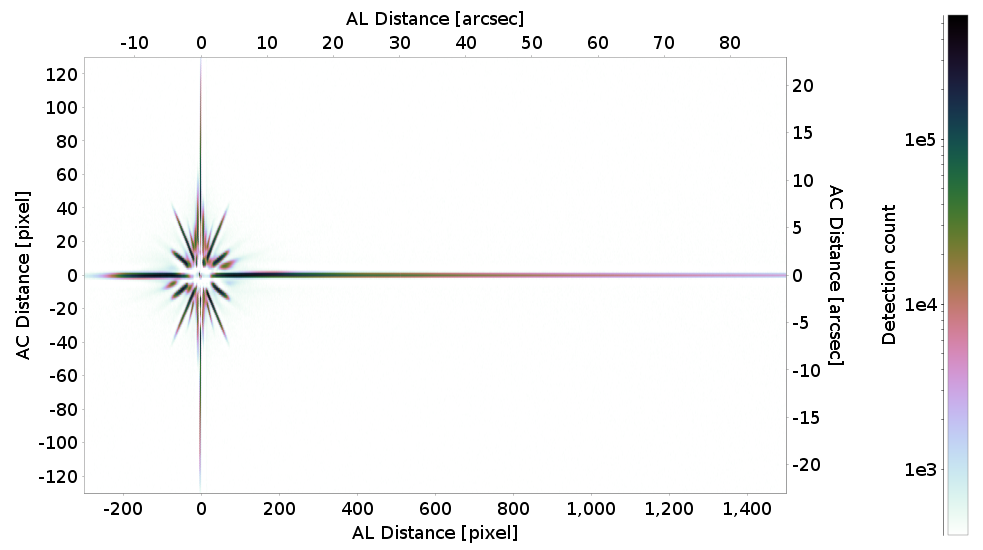
  Spurious detections around and along the diffraction spikes of sources brighter than about $G=16$. Detections are classified as spurious detections if they fall within a predefined set of regions and ranges of magnitude, centred on the bright source. These regions are determined from detection density maps as shown in Figure 3.16. For very bright objects ( mag), we even check the detections in the opposite field of view to catch spurious detections coming from unwanted light paths in the instrument.

• •

  Phantom detections; detections considered bright on board ( mag) but without the expected saturated samples in the centre of the SM window. They are caused by confusion of several bright sources by the on-board detection.

• •

  Spurious detections due to cosmic rays; rather bright detections in the SM but with very low signal in the remaining AF windows.

• •

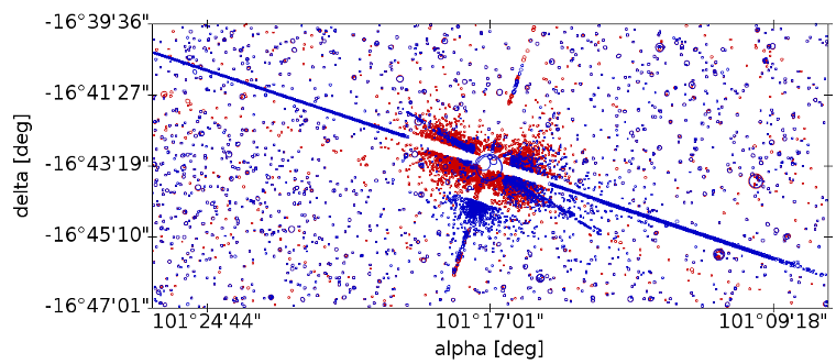
  Spurious detections around transits of the major planets (see Figure 3.18); as for the diffraction spikes, we use predefined regions and magnitude limits to identify the spurious detections.

• •

  Detections with odd flux signal profiles in the acquired windows, typically from diffraction spikes. This module analyses the window samples looking for meaningful point-like signals within the window core region.

• •

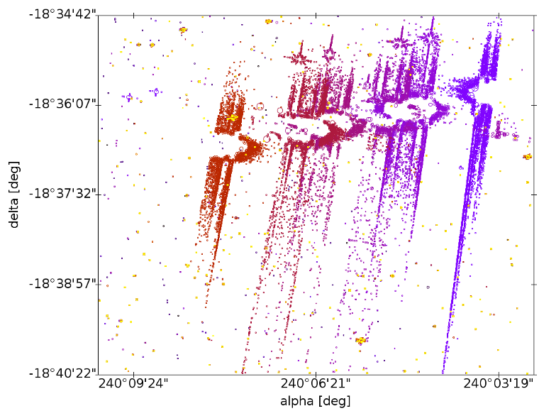
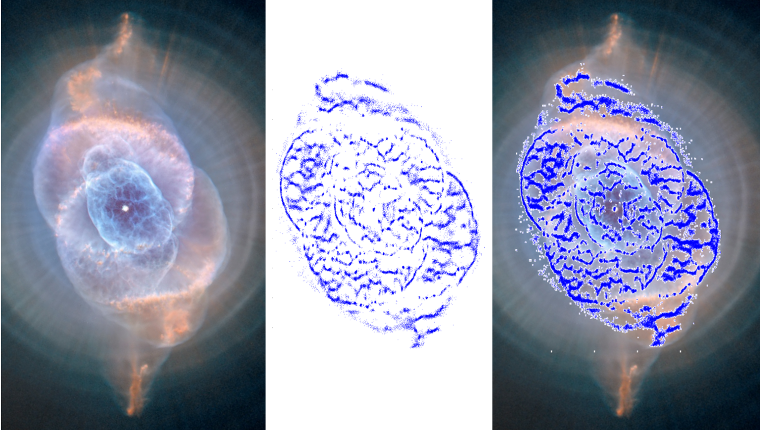
  Detections from extended and diffuse objects. Figure 3.19 shows that Gaia is actually detecting not only stars but also filamentary structures of high surface brightness. These detections are not strictly spurious, but require a special treatment. Their CCD images may differ too much from the expected PSF or LSF profile, in which case they may be classified as spurious detections.

• •

  Detections during periods with very noisy attitude solutions and spacecraft attitude issues.

Identifying spurious detections around fainter sources (down to 16 mag) is more difficult, since there are often only very few or none. In these cases, a multi-epoch treatment is required to know if a given detection is genuine or spurious, i.e., checking if more transits are in agreement and resolve to the same new source entry. These cases will be addressed in future data releases as the data reduction cycles progress and more information from that sky region is becoming available.

The spurious detections categories for which no countermeasures are yet in place include — amongst others — the spurious detections that happen randomly on the sky due to CCD defects and unwanted light paths. In general, these detections have poor astrometric and photometric parameters and are filtered out in the downstream processes.

For Gaia EDR3, the module analysing the image profiles has been reviewed in order to avoid rejecting detections of close pairs (separation below 400 mas). In Cycle-02 processing, there were indications that this module was picking out valid detections of close objects when more than one peak was visible and the window was not well centered on the brighter peak. Under these conditions, the module may classify incorrectly some detections affecting the quality of the final astrometric and photometric solutions. We estimate that a non-negligible fraction of these detections remains rejected in Gaia DR3 and furthermore some of these close sources may have few matched detections only. For this reason, a major update will be carried out in the next processing cycle to include the prompt identification of these detections and improve their treatment in the cross-match and subsequent pipelines (Torra et al. 2020).

Moreover, the total number of spurious detections in the Data Segments 0, 1 and 2 has increased from 10.737 million detections for Gaia DR2 to 11.294 million detections for Gaia EDR3. This increase is mainly explained by the new calibration used in the module in charge of the treatment of the diffraction spikes of bright objects.

This processing step is in charge of providing an initial list of source candidates for each individual detection.

The first step is the determination of the sky coordinates as described in Section 3.4.13. This step is executed in multiple tasks split by time interval blocks. All Gaia observations enter this step, with the exception of Virtual Objects, and data from dedicated calibration campaigns. Also, all the observations positively classified as spurious detections are filtered out.

Once the detection sky coordinates are available, these are compared with a list of sources. In this step, the observation-to-source matching, the sources that cover the sky seen by Gaia in the time interval of each task, are extracted from the Gaia catalogue. These sources are propagated with respect to parallax, proper motion, orbital motion, etc. to the relevant epoch.

The candidate sources are selected based on a pure angular distance criterion. The decision of only using distance was taken because the position of a source changes slowly and predictably, whereas other parameters such as the magnitude may change in an unpredictable way. Additionally, the initial Gaia catalogue is quite heterogeneous, exhibiting different accuracy levels and errors which suggest the need of a match criterion subjected to the provenance of the source data. In later stages of the mission, when the source catalogue is dominated by Gaia astrometry, this dependency can be removed and then the criterion should be updated to take advantage of the better accuracy of the detection in the along-scan direction. At that point, it will be possible to use separate along- and across-scan criteria, or use an ellipse with the major axis oriented across scan which will benefit the resolution of the most complex cases.

For Gaia DR3, as described in Torra et al. (2020), a match candidate radius of 5${}^{\mathrm{\prime \prime }}$was selected, balancing the wish to avoid the creation of too large groups (see  Section 3.4.13) on the one hand, and the objective to find some unknown high proper motion sources on the other hand. This value was chosen taking into account that Gaia completes a full scan of the sky in 6 months and that the fastest-moving star in Earth’s skies, Barnard’s Star, annually travels 10${.}^{\mathrm{\prime \prime }}$3. Note that, if a source is moving faster or the time gaps between consecutive scans are too large, some of its observations could end up in separated groups of detections. However, if several scans are grouped together, we should be able to determine a sufficiently good proper motion from the detections in one of the groups enforcing the regrouping of all its detections in the next cycle when the proper motion is available in the catalogue and applied when computing the candidate sources.

A special case is the treatment of solar system objects observations. The processing of these objects are the responsibility of CU4 (Section 1.2.2) and for this reason, no special considerations have been implemented in the cross-match. These observations will have Gaia Catalogue entries created on a daily basis by IDT and those entries will remain, so the corresponding detections will be matched again and again to their respective sources without any major impact on the other objects.

An additional processing may be required when detections without source candidates are left after the observation-to-source matching process. In principle, this situation should be rare since IDT has already treated all detections before IDU runs. However, unmatched detections may arise because of IDT processing failures, updates in the detection classification, updates in the source catalogue, or simply the usage of a more strict match criterion in IDU. Thus, this additional process is basically in charge of processing the unmatched detections and creating temporary sources as needed just to remove all the unmatched detections in a second run of the source-matching process. The new sources created by these tasks will ultimately be resolved (by confirmation or deletion) in the last cross-match step.

Summarising, the result of this first step is a set of MatchCandidates for the whole accumulated mission data. Each MatchCandidate corresponds to a single detection and contains a list of source candidates. Together with the MatchCandidates, an auxiliary table is produced to track the number of links created to each source, the SourceLinksCount table. Results are stored in a spatial-based structure using HEALPix (Górski et al. 2005), for convenience of the subsequent processing steps.

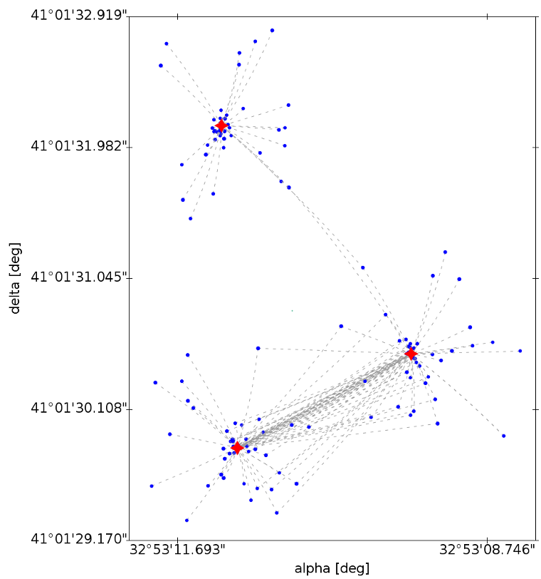
The sky partitioner task is in charge of grouping the results of the observation-to-source matching (Section 3.4.13) according to the source candidates provided for each individual detection (Torra et al. 2020). The purpose of this process is to create self-contained groups of MatchCandidates. The process starts loading all MatchCandidates for a given sky region. From the loaded entries, the unique list of matched sources is identified and the corresponding SourceLinksCount information is loaded. Once loaded, a recursive process is followed to find the isolated and self-contained groups of detections and sources. The final result of this process is a set of MatchCandidateGroups (as shown in Figure 3.20) where all the input observations are included. In summary, within a group, all observations are related to each other by links to source candidates. Consequently, sources present in a given group are not present in any other group.

As mentioned above in Section 3.4.13, the match radius used is large enough to keep detections of high proper motion stars in the same group of detections. However, this also increments the complexity of the groups and, occasionally, the groups produced in crowded areas could be too large and complex for the final resolution described below in Section 3.4.13. This complexity naturally increases when more data segments are added.

As explained in Torra et al. (2020), a source-candidates-crop algorithm has been implemented for Gaia EDR3 to limit the complexity of these groups. This new algorithm reduces the size of the largest groups by discarding some of the links between match candidates and source candidates, and recomputes the groups again. The links discarded are the optimum to reduce the size of the group, based on the detection-to-source distances and the total number of links to the same source candidate. By discarding these links, the original group is split into subgroups which can be processed later on.

After this process, each MatchCandidateGroup can be processed independently from the others as the observations and sources from two different groups are fully independent.

The final step of the cross-match is the most complex, namely resolving the final matches and consolidating the new sources. Three main cases need to be solved:

• •

  Duplicate matches: when two (or more) detections close in time are matched to the same source. This will typically be either newly resolved binaries or spurious double detections. In this case, two (or more) new sources are created and the source in the working catalogue is superseded by split.

• •

  Duplicate sources: when a pair of sources from the catalogue has never been observed simultaneously, thus never identifying two detections within the same time frame, but has the same matches. This can be caused by double entries in the working catalogue. In this case, a new source is created and the sources in the working catalogue are superseded by merge.

• •

  Unmatched observations: observations without any valid source candidate. In this case, a new source is created from scratch.

For the first cyclic processing and Gaia DR1, the resolution algorithm has been based on a nearest-neighbour solution in which the conflict between two given observations was resolved independently from the other observations included in the group. This was a simple and quick conflict resolution algorithm. However, this approach did not minimize the number of new sources created when more than two observations close in time had the same source as primary match.

The cross-match resolution algorithm in Gaia DR2 was based on a much more sophisticated algorithm. In particular, it uses tailored clustering and resolution algorithms in which all the relations between the observations contained in each group are taken into account to generate the best possible resolution.

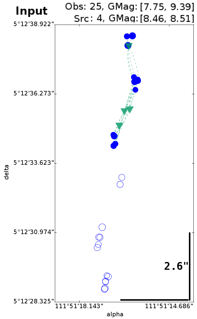
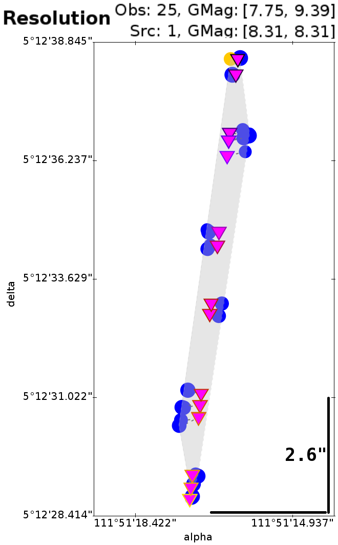
For Gaia EDR3 the model of cluster analysis is updated to improve the results for high proper motion sources and variables stars, using a hierarchical clustering algorithm with a linear source model (Torra et al. 2020). Moreover, it includes a post-processing algorithm to reduce the constraints of the clustering algorithm and the small number of sources with faulty significant negative and large parallax values listed in Gaia DR2 (see Gaia Collaboration et al. 2018a; Lindegren et al. 2018, appendix C). Finally, after the clustering solution, remaining spurious detection candidates are classified with a global spatial treatment using the cluster information in order to prevent the creation of new sources from spurious detections (Torra et al. 2020). Figure 3.21 shows an example of a high proper motion source that benefits from the updated clustering model.