4.3 Calibration models 4.3.5 Attitude model 4.3.7 Global parameters

4.3.6 Geometric instrument model

Author(s): Lennart Lindegren

Figure 4.11: Schematic illustration of the definition of observation lines in field angles.

The geometric instrument model (or astrometric calibration model) is an accurate description of the CCD layout in the Scanning Reference System (SRS; Section 4.1.3) $\mathsf{S}=[\boldsymbol{x}~{}\boldsymbol{y}~{}\boldsymbol{z}]$ , or equivalently in instrument angles $(\varphi,\zeta)$ or field angles $(f,\eta,\zeta)$ . The three systems are equivalent because a given direction $\boldsymbol{u}$ can be represented in either system by means of the relations

\mathsf{S}^{\prime}\boldsymbol{u}=\begin{bmatrix}u_{x}\\ u_{y}\\ u_{z}\end{bmatrix}=\begin{bmatrix}\cos\zeta\cos\varphi\\ \cos\zeta\sin\varphi\\ \sin\zeta\end{bmatrix}=\begin{bmatrix}\cos\zeta\cos(\eta+f\Gamma_{\text{c}})\\ \cos\zeta\sin(\eta+f\Gamma_{\text{c}})\\ \sin\zeta\end{bmatrix}

(4.116)

where $f=\text{sign}(u_{y})$ is the field index ( $f=+1$ in preceding field of view, $-1$ in following field of view) and $\Gamma_{\text{c}}=106\hbox{$.\!\!^{\circ}$}5$ is the conventional basic angle. Conversely, the $x y$ plane of the SRS and the origin of the along-scan (AL) instrument angle $\varphi$ are implicitly defined by the geometric instrument model, or more precisely by certain constraints imposed on the model. The geometrical instrument model is based on the calibration model described in Section 3.4 of Lindegren et al. (2012).

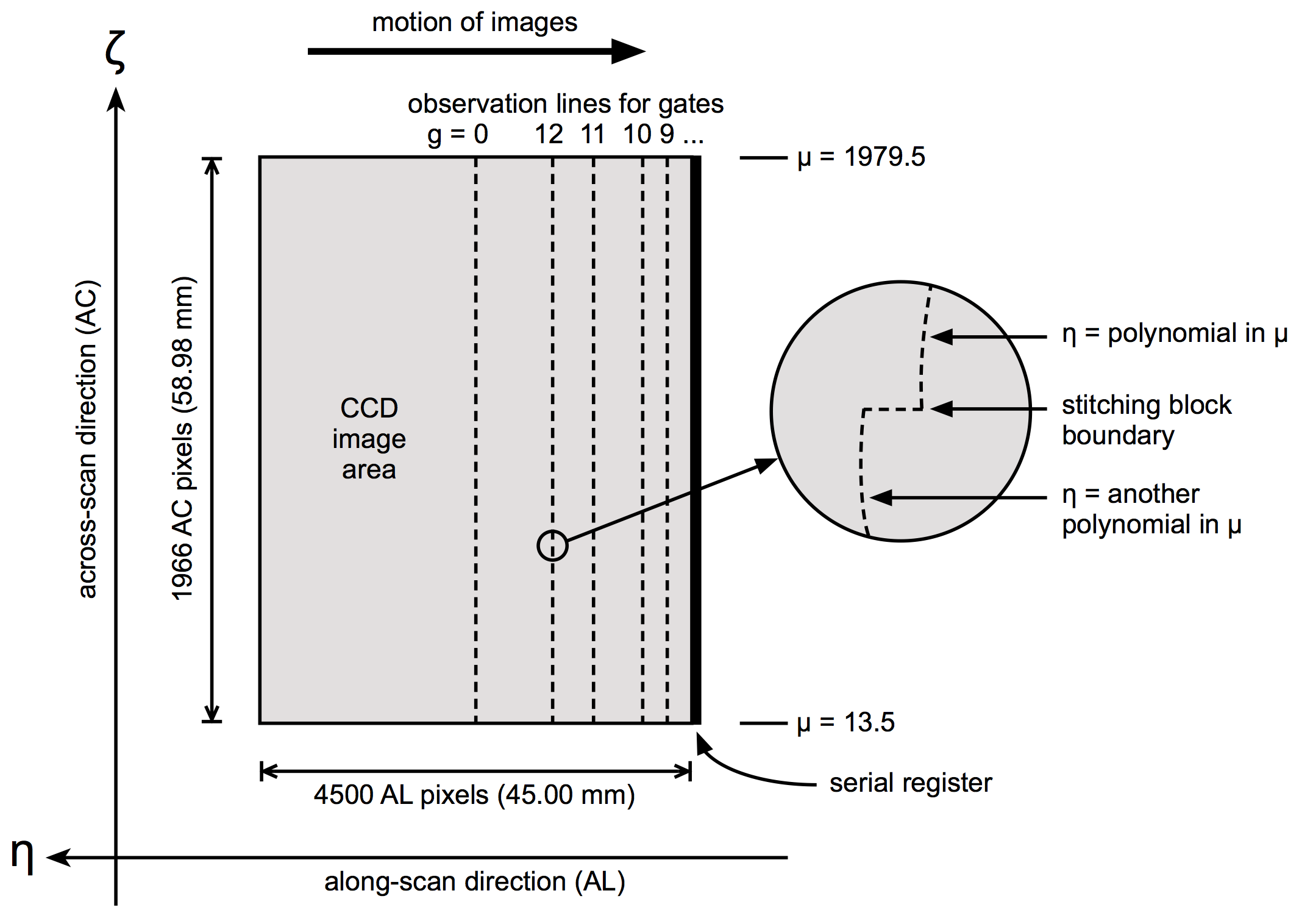
A central concept for the geometric instrument calibration is the observation line, which is an imaginary curve extending over the full width of the CCD image area in the across-scan (AC) direction (Figure 4.11). For ungated observations (gate index $g=0$ ), where all $\simeq\,$ 4500 AL pixels are used to integrate the image, the observation line is nominally situated $\simeq\,$ 2250 TDI lines prior to the serial register (see Table 1.3 for exact numbers). For gated observations using the first gate ( $g=12$ ), only the last $\simeq\,$ 2900 TDI lines are used for the integration, and the observation line is consequently situated $\simeq\,$ 1450 TDI lines prior to the serial register. The AC pixel coordinate $\mu$ is a continuous variable in the range $[13.5,\,1979.5]$ , with $\mu=14.0$ when the image is centrally located in the AC direction of the first pixel column (with the smallest AC field angle $\zeta$ ), and $\mu=1979.0$ when the image is centrally located in the AC direction of the last (1966th) pixel column.

The elementary astrometric measurement, obtained from the transit of a given source over a single (SM or AF) CCD, is the observation time $t_{\text{obs}}$ and AC pixel coordinate of the image, $\mu_{\text{obs}}$ . The observation time is calculated, in on-board time, as the read-out time of the reference pixel of the observation window, corrected for the AL offset of the image centroid from the reference pixel, minus the exposure mid-time offset for the relevant $g$ (Table 1.3). ( $t_{\text{obs}}$ is subsequently converted to TCB using the time ephemeris; see Section 4.1.3.) The observed AC pixel coordinate $\mu_{\text{obs}}$ is obtained by correcting the AC coordinate of the window reference pixel for the AC offset of the image centroid from the reference pixel, but is only available for observations using a two-dimensional window.

The optical design of the Gaia telescopes and the mechanical layout of the focal-plane assembly are such that the TDI lines of all the CCD are very nearly parallel to lines of constant AL field angle $\eta$ in the SRS. (This is a necessary condition for the TDI operation of all the CCDs using the same TDI period.) Thus, to a first approximation the observation lines are short segments of great-circle arcs with a fixed $\eta$ for a given CCD and gate. However, in reality the structure of an observation line is much more complex, as suggested by the ‘magnifying glass’ in Figure 4.11. For a given CCD/gate combination, the observation lines are different in the two fields of view, due to the optical distortions being different, and they vary with time due to thermal-mechanical changes in the optics and focal-plane assembly. Additional dependences (e.g, on window class $w$ ) are discussed below.

The observation line for a given combination of field index $f$ , CCD index $n$ (e.g., in the range 1 through 62 in the AF), gate $g$ , and window class $w$ is defined in parametric form as

\left.\begin{aligned} \displaystyle\eta&\displaystyle=\eta_{fngw}(\mu,\,t,\,% \dots)\\ \displaystyle\zeta&\displaystyle=\zeta_{fngw}(\mu,\,t,\,\dots)\end{aligned}% \quad\right\}\,,\quad 13.5\leq\mu\leq 1979.5\,.

(4.117)

Index $w$ refers to the window class (or sampling class) assigned to the observation by the on-board processing software, based on the on-board estimate of the $G$ magnitude; see Section 1.1.3 and Table 1.2 for details. Note that only eight of the gate settings, corresponding to $g=0$ , 12, 11, 10, 9, 8, 7, and 4 (see Table 1.3) are used in nominal operations. The astrometric calibration model for Gaia EDR3 used four sampling classes, corresponding to 0A, 0B, 1, and 2 in Table 1.2.

Since $\mu_{\text{obs}}$ is only available for observations in two-dimensional windows, the argument $\mu$ in Equation 4.117 should be the AC pixel coordinate of the image calculated from current source, attitude, and calibration parameters. The dependence on $\mu$ involves both large-scale effects, such as the slope and curvature of the observation line, medium-scale effects, for example caused by the stitch blocks, and small-scale effects that vary on a level of a few pixel columns or units in $\mu$ . The required precision in the calculated $\mu$ is therefore very modest ( $\sim\,$ 1 unit), and even a very preliminary set of parameters will be sufficient for this. However, for Gaia EDR3 an approximate $\mu$ was instead used, which for 1D windows was taken to be the centre of the window in the AC direction, and for 2D windows the AC coordinate obtained from the PSF fitting made by the IDU (Section 3.4.2).

The time argument $t$ in Equation 4.117 is the observation time $t_{\text{obs}}$ , which should here be understood as representing the slow variation of the observation lines with time, including for example the basic-angle variations — these are ‘slow’ (time scales of hours to years) in comparison with the precisions involved in measuring $t_{\text{obs}}$ , which are in the $\mu$ s range. The time dependence in Equation 4.117 must be able to accommodate both gradual and sudden changes of the instrument geometry. The former could for example be caused by ageing of the mechanical structure, variations in the thermal environment, and the progressive development of change transfer inefficiency in the CCD detectors. Sudden changes may happen spontaneously or in connection with planned operational events such as mirror decontaminations, telescope refocusing, and special calibration activities. The existence of sudden changes, whether they are planned or spontaneous, makes it necessary to have breakpoints (discontinuities) in the geometric model at specific times. The times of discontinuities are known for planned events but are in other cases only found by inspection of the actual data.

The time dependence is generally modelled by dividing the full time interval $[t_{0},t_{J}]$ covered by the instrument model into a set of $J$ contiguous time granules, such that the granule indexed by $j$ ( $j=0\dots J-1$ ) covers $t_{j}<t<j_{j+1}$ . Here, $t_{j}$ ( $j=0\dots J$ ) are the chosen breakpoints, with $t_{0}$ and $t_{J}$ at the beginning and end of the full time interval covered by the model. Within a granule the variation is modelled as a low-order polynomial. To ensure that the polynomial model is accurate enough within a granule, it may be necessary to insert additional breakpoints — not motivated by known discontinuities in the data — at suitable times to limit the size of the granules. Continuity conditions are never imposed across breakpoints.

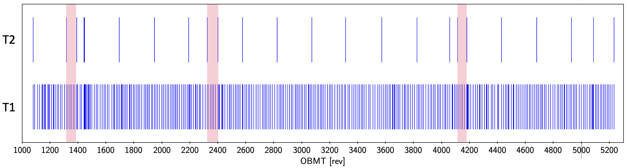
Different effects may require different time resolutions. Generally speaking, small-scale effects, representing mainly the internal structure of the CCDs, are stable over long times, while large-scale effects, depending on opto-mechanical variations, tend to vary significantly on much shorter time scales. The geometric instrument model uses several different time axes, each with its own granularity, or set of breakpoints. For practical reasons the time axes should be hierarchic in the sense that the breakpoints of a coarser time axis is a subset of the breakpoints of the finer time axis. For Gaia EDR3 two time axes are used: T1 with 310 granules of typically 3 d duration, and T2 with 19 granules of typically about 63 d duration (Figure 4.12). However, in many cases the exact boundaries were adjusted to coincide with the start or end times of data gaps, so as not to create unnecessarily short granules. T1 is used for the rapidly changing large-scale distortion, while T2 is used for the more slowly evolving effects.

Figure 4.12: Time axes T1 and T2 used for the geometric instrument model in Gaia EDR3. The vertical blue lines mark the breakpoints. The first and last lines mark the beginning and end of the time interval used in the primary astrometric solution and for all astrometric results. The pink intervals are the gaps during and after decontaminations. In the gaps there are some empty granules on the T1 axis; these are disregarded in the calibration.

The dots ( $\dots$ ) in Equation 4.117 represent possible dependences on additional continuous variables such as the colour and magnitude of the source at the time of observation (COMA terms; see Section 4.3.6).

The functions in Equation 4.117 are written as sums of a fixed reference calibration $\eta_{ng}^{(0)}(\mu)$ , $\zeta_{fng}^{(0)}(\mu)$ , calculated from the nominal layout of the CCDs and gates, and a number of ‘effects’, which in turn are linear combinations of basis functions with the calibration parameters as coefficients. The generic expressions are

\left.\begin{aligned} \displaystyle\eta_{fngw}(\mu,t,\dots)&\displaystyle=\eta% _{ng}^{(0)}(\mu)+\sum_{i}E^{\text{AL}}_{i}(o)+\frac{f}{2}\Delta\Gamma(t)+% \delta\eta(o)\\ \displaystyle\zeta_{fngw}(\mu,t,\dots)&\displaystyle=\zeta_{fng}^{(0)}(\mu)+% \sum_{i}E^{\text{AC}}_{i}(o)\end{aligned}\quad\right\}\,,

(4.118)

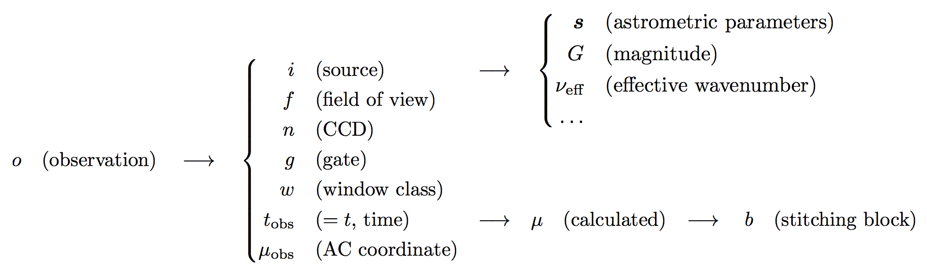
where $E^{\text{AL}}_{i}$ and $E^{\text{AC}}_{i}$ are the AL and AC calibration effects detailed in Section 4.3.6 and Section 4.3.6. The effects are here formally written as functions of the observation index $o$ , from which all other required indices and arguments can be obtained (Figure 4.13). The AL component of Equation 4.118 contains two further terms that are not discussed in this section. The first one contains the basic-angle correction $\Delta\Gamma(t)$ derived from the analysis of BAM data (Section 4.2.4). The other term, $\delta\eta(o)$ , contains the sum of the AL instrument effects derived as part of the global model in Section 4.3.7.

Figure 4.13: Quantities derived from the observation index $o$ .

The AL and AC calibration functions for effect $i$ are written as linear combinations of basis functions depending on several different variables implicitly defined by $o$ . The variables are of two kinds: discrete variables (indices and flags) and continuous variables (such as $t$ , $\mu$ , and $\nu_{\text{eff}}$ ).

All effects are assumed to depend on indices $j$ (granule index for the relevant time axis), $f$ (field-of-view index), and $n$ (CCD index); depending on the effect it could also depend on $g$ (gate), $w$ (window class), and the stitch-block index $b$ calculated as

b=\text{floor}\left(\frac{\mu+128.5}{250}\right)\,.

(4.119)

Indices $l$ and $m$ are used to describe the dependences on $\mu$ (within a given CCD $n$ ) and $t$ (within a given granule $j$ ) by means of shifted Legendre polynomials $\tilde{P}_{n}(x)=P_{n}(2x-1)$ , where $P_{n}(x)$ are the normal (non-shifted) Legendre polynomials. The shifted Legendre polynomials are orthogonal on $[0,\,1]$ and reach $\pm 1$ at the end points. The first four polynomials are

\left.\begin{aligned} \displaystyle\tilde{P}_{0}(x)&\displaystyle=1\\ \displaystyle\tilde{P}_{1}(x)&\displaystyle=2x-1\\ \displaystyle\tilde{P}_{2}(x)&\displaystyle=6x^{2}-6x+1\\ \displaystyle\tilde{P}_{3}(x)&\displaystyle=20x^{3}-30x^{2}+12x-1\end{aligned}% \quad\right\}\,.

(4.120)

The joint dependence $\mu$ and $t$ is written as linear combinations of basis functions that are products of the shifted Legendre polynomials of degree $l$ and $m$ , i.e.

K_{lm}(\tilde{\mu},\tilde{t})=\tilde{P}_{l}(\tilde{\mu})\tilde{P}_{m}(\tilde{t% }\,)\,,

(4.121)

where

\tilde{\mu}=\frac{\mu-\mu_{\text{min}}}{\mu_{\text{max}}-\mu_{\text{min}}}

(4.122)

is the normalised AC pixel coordinate, with the limits $\mu_{\text{min}}=13.5$ and $\mu_{\text{max}}=1979.5$ (Figure 4.11), and

\tilde{t}=\frac{t-t_{j}}{t_{j+1}-t_{j}}

(4.123)

the normalised time within granule $j$ , with $t_{j}\leq t<t_{j+1}$ .

Additional dependencies on $\nu_{\text{eff}}$ (effective wavenumber), $G$ (magnitude), $S$ (saturation flag), $\phi$ (subpixel phase), $\Delta t$ (time since last charge injection), and $\dot{\zeta}$ (across-scan rate) are described as they are introduced below. The specific functions in effect $i$ are generically written as $\Psi^{(i)}_{k}(o)$ , where $k=0$ , 1, $\dots$ for the different functions that may be required for the effect.

The calibration requirements are much stricter AL than AC, and the models for $\eta_{fngw}(\mu,\,t,\,\dots)$ and $\zeta_{fngw}(\mu,\,t,\,\dots)$ are separately described hereafter. The particular models described here are the ones used for Gaia EDR3 (see Section 3.3 in Lindegren et al. 2021); more elaborate models will be used for subsequent releases.

AL geometric instrument model

The AL geometric instrument model is the sum of the seven effects enumerated below.

1.

AL large-scale geometric ( $i=1$ ) describes the relatively rapid variations of the large-scale distortion, and therefore uses the time axis T1 with the smallest granules (typically 3 days). It depends on the field index, CCD index, and window class, but is the same for all gates and blocks. It assumes a quadratic dependence on $\mu$ and a linear dependence on $t$ within a granule, and is therefore a linear combination of four basis functions,

$\begin{split}\displaystyle E^{\text{AL}}_{1}(o)&\displaystyle=\sum_{lm\,=\,00,% \,10,\,20,\,01}\Delta\eta^{(1)}_{lmjfnw}K_{lm}(\tilde{\mu},\tilde{t})\end{split}$ (4.124)

with a total of $4\times 310\times 2\times 62\times 4=615\,040$ calibration parameters.
2.

AL medium-scale gate ( $i=2$ ) describes the slowly varying joint dependence on gate ( $g$ ) and stitch block ( $b$ ). The times axis is T2 with granules of typically 63 days. The model assumes a linear dependence on $\mu$ for each gate/block combination, and no time variation within a granule. The effect is therefore a linear combination of two basis functions,

$\begin{split}\displaystyle E^{\text{AL}}_{2}(o)&\displaystyle=\sum_{lm\,=\,00,% \,10}\Delta\eta^{(2)}_{lmjfngb}K_{lm}(\tilde{\mu},\tilde{t})\,,\end{split}$ (4.125)

with a total of $2\times 19\times 2\times 62\times 8\times 9=339\,264$ calibration parameters.
3.

AL large-scale colour ( $i=3$ ) describes the slowly varying dependence on colour ( $\nu_{\text{eff}}$ ), using times axis T2 with granules of typically 63 days and a linear variation with time in each granule. The model assumes that the effect is different for each window class ( $w$ ) but the same for all $\mu$ within a CCD. The effect is therefore a linear combination of two basis functions,

$\begin{split}\displaystyle E^{\text{AL}}_{3}(o)&\displaystyle=\sum_{lm\,=\,00,% \,01}\Delta\eta^{(3)}_{lmjfnw}K_{lm}(\tilde{\mu},\tilde{t})\,\Psi_{0}^{(3)}(o)% \,,\end{split}$ (4.126)

where $\Psi_{0}^{(3)}(o)=\nu_{\text{eff}}-\nu_{\text{eff}}^{\text{def}}$ . This effect has a total of $2\times 19\times 2\times 62\times 4=18\,848$ calibration parameters.
4.

AL large-scale saturation ( $i=4$ ) describes the AL shift associated with partially saturated images. These are identified by a flag set in the pre-processing when the raw observed sample exceeds a pre-defined threshold for the CCD column and sample binning. This effect is only used for window classes WC0a and WC0b (that is for 2D windows) and is taken to be constant within a granule of T2, independent of $\mu$ , but different in WC0a and WC0b. The effect therefore consists of a single basis function,

$\begin{split}\displaystyle E^{\text{AL}}_{4}(o)=\Delta\eta^{(4)}_{00jfnw}K_{00% }(\tilde{\mu},\tilde{t})\,\Psi_{0}^{(4)}(o)\,,\end{split}$ (4.127)

where $\Psi_{0}^{(4)}(o)=1$ if the saturation flag is set for observation $o$ , otherwise $0$ . This effect has a total of $1\times 19\times 2\times 62\times 2=4712$ calibration parameters.
5.

AL large-scale subpixel ( $i=5$ ) describes a systematic AL shift that is a periodic function of the subpixel phase $\phi$ . The subpixel phase is $2\pi$ times the fractional part of the observation time expressed in TDI periods. This effect is taken to be constant within a granule of T2, independent of $\mu$ , but different for each windo class. The periodic dependence requires the use of two basis functions,

$\begin{split}\displaystyle E^{\text{AL}}_{5}(o)=\sum_{k=0}^{1}\Delta\eta^{(5)}% _{00jfnwk}K_{00}(\tilde{\mu},\tilde{t})\,\Psi_{k}^{(5)}(o)\,,\end{split}$ (4.128)

where $\Psi_{0}^{(5)}(o)=\cos\phi$ and $\Psi_{1}^{(5)}(o)=\sin\phi$ . This effect has a total of $1\times 19\times 2\times 62\times 4\times 2=18\,848$ calibration parameters.
6.

AL large-scale CTI ( $i=6$ ) describes the shift caused by charge transfer inefficiency (CTI) as a function of the time $\Delta t$ since the last charge injection. In the CCDs of the astrometric field, charge injections made at regular intervals of 2000 TDI periods (about 2 s) mitigate CTI by keeping some charge traps filled (see Section 1.3.4 and Section 3.4.8), but as the traps release their charges the effect tends to increase with $\Delta t$ until the next charge injection. The AL CTI effect is modelled as a superposition of four exponential functions with $e$ -folding times $\tau_{k}=10$ , 100, 500, and 2000 TDI periods ( $k=0,~{}1,~{}2,~{}4$ ). The effect is assumed to be different for each window class and constant in a time granule on T2. The effect is a linear combination of four basis functions,

$\begin{split}\displaystyle E^{\text{AL}}_{6}(o)&\displaystyle=\sum_{k=0}^{3}% \Delta\eta^{(6)}_{00jfnwk}K_{00}(\tilde{\mu},\tilde{t})\,\Psi_{k}^{(6)}(o)\,,% \end{split}$ (4.129)

where $\Psi_{k}^{(6)}(o)=a_{k}-\exp(-\Delta t/\tau_{k})$ . The constants $a_{k}=(\tau_{k}/2000)[1-\exp(-2000/\tau_{k})]$ are chosen to make $\Psi_{k}^{(6)}(o)$ on average zero for $0\leq\Delta t\leq 2000$ TDI periods. Because observations are statistically more or less uniformly distributed in $\Delta t$ it means that the mean AL displacement produced by the CTI is not taken out by this effect, only its variation with $\Delta t$ . This effect has a total of $1\times 19\times 2\times 62\times 4\times 4=37\,696$ calibration parameters.
7.

AL large-scale AC rate ( $i=7$ ) represents the AL shift proportional to the amount of AC smearing produced by the AC rate $\dot{\zeta}$ . This effect is only used for observations in window class WC0b using gates 11, 12, and 0 (the ‘long’ gates, that is with integration times of at least about 2 s). The effect is taken to be different in each time granule on the T2 axis. It consists of a single basis function,

$\begin{split}\displaystyle E^{\text{AL}}_{7}(o)&\displaystyle=\Delta\eta^{(7)}% _{00jfn}K_{00}(\tilde{\mu},\tilde{t})\,\Psi_{0}^{(7)}(o)\,,\end{split}$ (4.130)

where $\Psi_{0}^{(7)}(o)=|\dot{\zeta}|$ . This effect has a total of $1\times 19\times 2\times 62=2356$ calibration parameters.

Counting all five effects, the number of AL calibration parameters is 1 036 764.

AC geometric instrument model

The AC geometric instrument model is similar to the AL model, except that time axis T2 with a typical granule size of 63 days is used for all the effects, that the gate effect is dependence of $\mu$ and $b$ , and that there is no dependence on subpixel phase $\phi$ , time since charge injection $\Delta t$ , and AC rate $\dot{\zeta}$ . On the other hand, the AC calibration includes a dependence on magnitude $G$ . The AC calibration requires 2D windows, so it is only relevant for window classes WC0a and WC0b. The model is the sum of the five effects enumerated below ( $i=8$ to 12).

8.

AC large-scale geometric ( $i=8$ ) describes the variations of the large-scale distortion, using time axis T2. It depends on the field, CCD, and window class indices, but is the same for all gates. It assumes a quadratic dependence on $\mu$ and a linear dependence on $t$ within a granule, and is therefore a linear combination of four basis functions,

$\begin{split}\displaystyle E^{\text{AC}}_{8}(o)=\sum_{lm\,=\,00,\,10,\,20,\,01% }\Delta\zeta^{(8)}_{lmjfnw}K_{lm}(\tilde{\mu},\tilde{t})\,,\end{split}$ (4.131)

with a total of $4\times 19\times 2\times 62\times 2=18\,848$ calibration parameters.
9.

AC medium-scale gate ( $i=9$ ) describes the dependence on gate ( $g$ ), using times axis T2. The model assumes a constant offset for each gate within a time granule and CCD. The effect is therefore

$\begin{split}\displaystyle E^{\text{AC}}_{9}(o)=\Delta\zeta^{(9)}_{00jfng}K_{0% 0}(\tilde{\mu},\tilde{t})\,,\end{split}$ (4.132)

with a total of $1\times 19\times 2\times 62\times 8=18\,848$ calibration parameters.
10.

AC large-scale colour ( $i=10$ ) describes the dependence on effective wavenumber $\nu_{\text{eff}}$ depending on window class ( $w$ ), using times axis is T2. The model assumes no variation with $\mu$ or $t$ within a CCD and granule. The effect is therefore

$\begin{split}\displaystyle E^{\text{AC}}_{10}(o)&\displaystyle=\Delta\zeta^{(1% 0)}_{00jfnw}K_{00}(\tilde{\mu},\tilde{t})\,\Psi_{0}^{(10)}(o)\,,\end{split}$ (4.133)

where $\Psi_{0}^{(10)}(o)=\nu_{\text{eff}}-\nu_{\text{eff}}^{\text{def}}$ . The effect has a total of $1\times 19\times 2\times 62\times 2\times 1=4712$ calibration parameters.
11.

AC large-scale magnitude ( $i=11$ ) describes the dependence on magnitude $G$ depending on window class ( $w$ ), using times axis is T2. The effect is only used for ungated observations ( $g=0$ ) The model assumes no variation with $\mu$ or $t$ within a CCD and granule. The effect is therefore

$\begin{split}\displaystyle E^{\text{AC}}_{11}(o)&\displaystyle=\Delta\zeta^{(1% 1)}_{00jfnw}K_{00}(\tilde{\mu},\tilde{t})\,\Psi_{0}^{(11)}(o)\,,\end{split}$ (4.134)

where $\Psi_{0}^{(11)}(o)=G-12.6$ . The effect has a total of $1\times 19\times 2\times 62\times 2\times 1=4712$ calibration parameters.
12.

AC large-scale saturation ( $i=12$ ) describes the image shift for saturated images. The model is the same as for the AL large-scale saturation effect,

$\begin{split}\displaystyle E^{\text{AC}}_{12}(o)=\Delta\zeta^{(12)}_{00jfnw}K_% {00}(\tilde{\mu},\tilde{t})\,\Psi_{0}^{(12)}(o)\,,\end{split}$ (4.135)

where $\Psi_{0}^{(12)}(o)=1$ if the saturation flag is set for observation $o$ , otherwise $0$ . This effect has a total of $1\times 19\times 2\times 62\times 2=4712$ calibration parameters.

In total there are 51 832 AC calibration parameters.

Constraints

In the astrometric solution for Gaia, constraints may be used to eliminate degeneracies among the various kinds of parameters: source (S), attitude (A), calibration (C), and global (G) parameters. Such constraints are introduced solely in order to make the parameters (or subsets of them) uniquely determinable, but they will never in any way ‘force’ the solution against the data.

To clarify exactly what this means, consider that the astrometric solution essentially solves a weighted least-squares solution by minimising some quantity $Q(\boldsymbol{x})$ for the given data. Here $\boldsymbol{x}$ is the vector of all the parameters or unknowns. A valid solution $\boldsymbol{\hat{x}}$ is such that $Q(\boldsymbol{\hat{x}})\leq Q(\boldsymbol{x})$ for all $\boldsymbol{x}$ . (Here we assume that the problem is linear, i.e. we take $\boldsymbol{x}$ to be the correction to a preliminary estimate of the parameters, and consider only a limited region in solution space where $\eta$ and $\zeta$ vary linearly with $\boldsymbol{x}$ .) If $\boldsymbol{\hat{x}}$ is a valid solution and there exists a non-zero vector $\boldsymbol{v}$ such that $\boldsymbol{\hat{x}}+\alpha\boldsymbol{v}$ is also a valid solution for any scalar $\alpha$ , then the problem is degenerate with respect to $\boldsymbol{v}$ , and $\boldsymbol{v}$ is a null vector of the problem. The degeneracy can be removed by applying a constraint of the form $\boldsymbol{v}^{\prime}\boldsymbol{x}=0$ , which is equivalent to selecting the particular solution with $\alpha=-(\boldsymbol{v}^{\prime}\boldsymbol{\hat{x}})/(\boldsymbol{v}^{\prime}% \boldsymbol{v})$ . Since this is still a valid solution, the constraint does not increase $Q$ , i.e. it does not work against the data.

A well-known example of degeneracy in the astrometric solution concerns the celestial reference frame (Section 4.3.2). If the positions of all sources are changed by a solid rotation of the reference frame by some (small) angle around an arbitrary direction, and the attitude parameters are correspondingly changed, the modified source and attitude parameters will fit the data equally well as the original values. In this example only the source and attitude parameters are modified, while the calibration and global parameters are not changed. The degeneracy can therefore be described as a source–attitude (SA) degeneracy. It is removed by the frame rotator implementing constraints based on external information on quasars.

Other kinds of degeneracies involve other subsets of the parameters, e.g. calibration–attitude (CA), calibration–source (CS), calibration–calibration (CC), and even calibration–attitute–source (CAS) degeneracies. Obviously only degeneracies involving the source parameters directly affect the astrometric results, while others (for example CA and CC) may affect the convergence of the iterative solution. To map the full spectrum of degeneracies relevant for a given set of models is a very complex problem that has not yet been satisfactorily solved.

For Gaia EDR3 the basic CA constraints enforced by the calibration update of the AGIS solution are, in the AL direction,

\sum_{f}\sum_{n}\Delta\eta^{(1)}_{00jfnw}=0

(4.136)

applied to window class WC1 (that is, for $G\simeq 16$ –16 mag) in every time granule $j$ on the T1 axis, and in the AC direction

\sum_{n}\Delta\zeta^{(8)}_{00jfnw}=0

(4.137)

applied to window class WC0a and WC0b (that is, for $G\lesssim 13$ mag) for every combination of $j$ and $f$ , where $j$ is the time granule on the T2 axis. Effectively, Equation 4.136 defines the origin of the AL instrument angle $\varphi$ in Equation 4.116 by requiring that the mean displacement of the observation lines in the AL direction from their nominal locations should be zero at all times, when averaged over both fields of view and the 62 CCDs of the AF. Similarly, Equation 4.137 defines the origin of $\zeta$ separately in each field by requiring that the mean displacement in the AC direction from the nominal locations should be zero at all times, and in each field of view, when averaged over the 62 CCDs of the AF. At any time there are thus three constraints, one AL and two AC, that together define the $x y z$ axes of the SRS (Section 4.1.1): the AC constraints define the orientation of the $x y$ plane, and the AL constraint defines location of the $x$ axis in that plane.

The specifications of effects 2 (AL medium-scale gate) and 9 (AC large-scale gate) permit the fiducial lines of all eight gates to be displaced by the same amount, which would be equivalent to the large-scale geometric calibration. Moreover, effect 2 contains a linear dependence on $\mu$ per stitch block ( $b$ ), which could also represent the components in effect 1 that are linear in $\mu$ . These degeneracies require CC constraints to prevent that the corresponding calibration parameters develop uncontrollably in the AGIS iterations. This is achieved by applying a constraint of effects 2 and 9 for ungated observations ( $g=0$ ), such that they are orthogonal to the components in effect 1 with $lm=00$ and 10.

Other effects are, as far as possible, formulated in such a way that they do not require additional CC constraints. This is achieved, for example, by the use of Legendre polynomials for the dependencies on $\mu$ and $t$ in the functions $K_{lm}(\tilde{\mu},\tilde{t})$ , and of the $\cos\phi$ and $\sin\phi$ basis functions for effect 5 (AL large-scale subpixel). Given the approximately uniform distribution of observations in $\mu$ , $t$ , and $\phi$ , these functions are not only linearly independent (thus requiring no special CC constraint) but uncorrelated to a high degree in the astrometric solution, which improves the convergence.

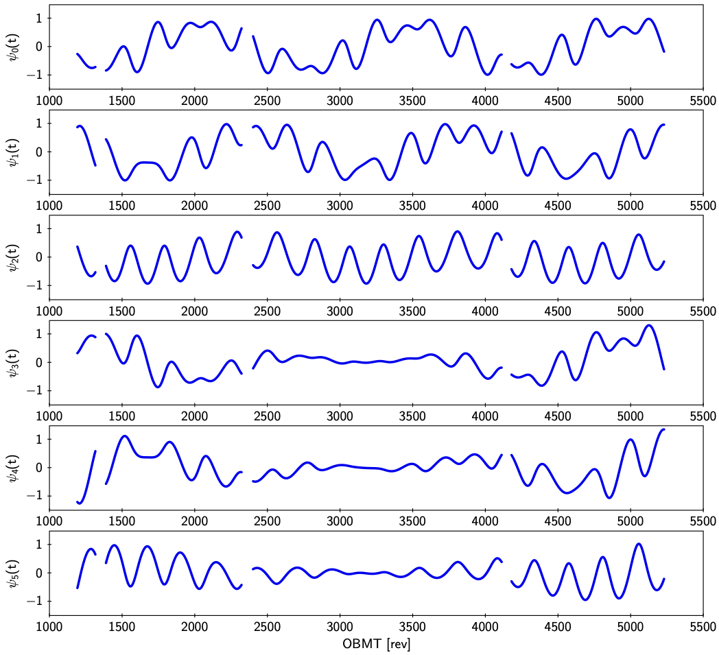
Degeneracies of the calibration–source (CS) kind may appear for AL effects that depend on variables that divide the sources into well separated subsets. An example is effect 3, depending on the colour ( $\nu_{\text{eff}}$ ) of the source. Unlike the variables $\mu$ , $t$ , or $\phi$ discussed above, which always have a good spread among the observations of a given source, $\nu_{\text{eff}}$ is (at least in Gaia EDR3) always the same in every observation of the source. The CS degeneracy could then result in a solution where positions and proper motions of sources are expressed in different reference frames, depending on the colour of the sources. It could happen, for example, that the reference frames of red and blue sources are slowly rotating with respect to each other. This kind of degeneracy can be understood by considering the observational effects of a small change in the reference frame orientation, given by the vector $\boldsymbol{\varepsilon}$ in Equation 4.92. At time $t$ , when the $z$ (nominal spin) axis of the SRS is pointing along the unit vector $\boldsymbol{z}(t)$ and the frame orientation error is $\boldsymbol{\varepsilon}(t)$ , the corresponding shift in the AL field angle is $\psi(t)=\boldsymbol{z}(t)^{\prime}\boldsymbol{\varepsilon}(t)$ . If the AL calibration allows a time variation of this form, it cannot be observationally distinguished from a frame orientation error by $\boldsymbol{\varepsilon}(t)$ . However, $\psi(t)$ cannot be an arbitrary function of time. The axis pointing $\boldsymbol{z}(t)$ is determined by the scanning law, and the standard model of stellar motion (Section 4.1.4) only allows frame orientation errors of the form in Equation 4.93, with six degrees of freedom. Consequently $\psi(t)$ also has six degrees of freedom, and can be written as a linear combination of the six basis functions $\psi_{k}(t)$ shown in Figure 4.14. (The displayed functions are $z_{X}(t)$ , $z_{Y}(t)$ , $z_{Y}(t)$ , $z_{X}(t)(t-2016.0)$ , $z_{Y}(t)(t-2016.0)$ , and $z_{Z}(t)(t-2016.0)$ , where $[z_{Y},z_{Y},z_{Z}]$ are the rectangular components of $\boldsymbol{z}$ in the ICRS.) All sources cannot be shifted by the same function $\psi(t)$ , for that would be picked up and corrected by the frame rotator, but it is possible for different subsets of the sources to be shifted relative to each other in proportion to $\psi(t)$ , if the net effect sensed by the frame rotator is zero. The chromaticity modelling in Equation 4.126 is linear in $\nu_{\text{eff}}$ , and if the CS degeneracy of this effect creates systematic errors in the reference frame, they will also be linear in $\nu_{\text{eff}}$ .

The CS degeneracy discussed above required that the calibration variable ( $\nu_{\text{eff}}$ ) separates the sources into disjoint subsets. The use of different window classes and gates, depending mainly on the magnitude, also tends to separate the sources into different subsets, although not very strict because many sources obtain observations in multiple window classes or gates. In principle this mixing should prevent a complete CS degeneracy, but the near-degeneracy could still create problems in the solution that need to be handled. The problems could manifest themselves in a systematic difference of the reference frame as a function of window class and gate used, that is essentially as a function of the $G$ magnitude.

In AGIS there are different ways by which recognised degeneracies can be handled: (i) ideally the calibration model should be formulated in such a way that there are no degeneracies; (ii) otherwise the corresponding constraints should be introduced in the calibration model; (iii) in some cases the degeneracy may be handled by applying a post-solution correction to the data. The first has been a guiding principle when designing the basic geometric instrument model for Gaia. The second is exemplified by the CA constraints in Equation 4.136 and Equation 4.137, and the third by the frame rotator (Section 4.3.2). For the degeneracies or near-degeneracies of the CS kind, all three methods have been used for Gaia EDR3, although in no case completely successfully.

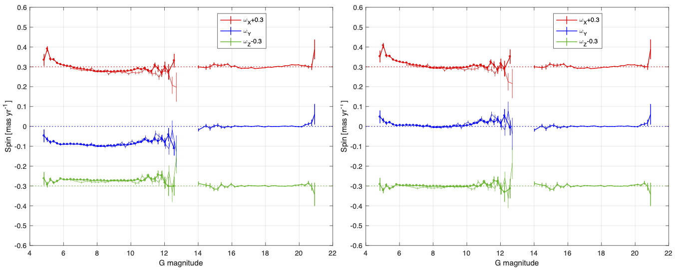
From Figure 4.14 it can be seen that the $\psi$ functions tend to oscillate with a period equal to the precession period of the nominal scanning law, $365.25/5.8\simeq 63$ d (Section 1.1.4). By selecting a granule size for time axis T2 close to 63 d (Figure 4.14) for calibration effects 2 (gate) and 3 (colour), their tendency to develop significant $\psi$ -like variations is much reduced. This can be seen as an approximation to method (i) above. For the large-scale geometric calibration (effect 1), which uses time axis T1 with a much higher time resolution, method (ii) was instead used to prevent that the different window classes define their separate reference frames. This appears to have been very effective for ensuring the continuity of the reference frame across the WC1/WC2 boundary at $G\simeq 16$ : as can be seen in the left panel of Figure 4.15 there is no significant change at that magnitude in the spin derived from the proper motions of quasars. However, the same plot clearly shows that the procedure was less successful at the WC0/WC1 boundary at $G\simeq 13$ : here a discontinuity of about 0.1 mas yr ${}^{-1}$ was seen in the spin of the preliminary primary solution. In this situation it was exceptionally decided to resort to method (iii): an ad hoc correction was applied to the calibration parameters for effect 1 of window classes WC0a and WC0b towards the end of the iteration sequence (see Lindegren et al. 2021 for details). The correction corresponds to a spin of the the bright reference frame by $\boldsymbol{\omega}=[-0.0166,\,-0.0950,\,+0.0283]^{\prime}$ mas yr ${}^{-1}$ . As shown in the right panel of Figure 4.15 this successfully brought the proper motions of the bright sources into agreement with the Hipparcos reference frame at epoch J1991.25. However, at that epoch the uncertainty of the alignment of the Hipparcos reference frame with the ICRS was about 0.6 mas per axis, and the bright reference frame of Gaia EDR3 consequently still has a systematic uncertainty of the order of $(0.6~{}\text{mas})/(24.75~{}\text{yr})\simeq 0.024$ mas yr ${}^{-1}$ per axis.

Figure 4.14: Psi functions for the calibration–reference frame degeneracy. An AL calibration effect that can be expressed as a linear combination of the six functions $\psi_{k}(t)$ ( $k=0$ , 1, $\dots$ , 5) cannot be distinguished from a time-dependent orientation error of the reference frame. The three breaks along the time axis represent the gaps in the astrometric data due to the decontaminations.

Figure 4.15: Spin of the primary AGIS solution before (left) and after (right) applying the *ad hoc* correction to the bright reference frame. For $G>14$ mag the spin was determined directly from the proper motions of quasars. For $G<13$ the spin was estimated from a comparison of the proper motions of Hipparcos and Tycho-2 stars in the primary AGIS solution with their proper motions calculated from the position differences between the AGIS solution at epoch J2016.0, and the Hipparcos (van Leeuwen 2007a) and Tycho-2 (Høg et al. 2000) catalogues at epoch J1991.25. Thick and thin lines are for the Hipparcos and Tycho-2 stars.

COMA terms

The geometric instrument model described in Section 4.3.6 and Section 4.3.6 contains terms depending on colour ( $\nu_{\text{eff}}$ ) and magnitude ( $G$ ) through effects 3, 10, and 11, the so-called COMA terms. They are needed because the location and shape of a point-source image, as seen by Gaia, in general depend on the colour of the object (e.g. due to wavelength-dependent diffraction effects in the optics) and its magnitude (e.g. due to charge transfer inefficiency in the CCD, which depends on the flux level). As described in Section 4.4.6, the intention is that COMA terms should eventually not be needed in the astrometric solution, namely when these effects are fully accounted for in the LSF and PSF calibrations. While this is not necessary for the processing of simple objects such as single stars, it will greatly simplify the (future) processing of more complex objects, and the purpose of this section is to explain the rationale for the adopted strategy. For simplicity the subsequent discussion focuses on the chromatic terms, although similar considerations apply to the magnitude effects.

In the calibration model for Gaia EDR3 there are additional effects, apart from the ones depending on $\nu_{\text{eff}}$ and magnitude $G$ , that should eventually be taken out by the LSF and PSF calibrations at IDU level. These are the dependencies on saturation (effects 3 and 12), subpixel position (effect 5), CTI (effect 6), and AC rate (effect 7). These are also counted to the COMA terms, although the simpler designation is retained. In the following discussion we disregard these additional effects, although they are actually treated in the same way as the colour- and magnitude-dependent effects.

Figure 4.16: Observation lines in local plane coordinates (LPC). (a) A point source S without proper motion or parallax is observed in three scans, with observation times $t_{\text{obs,1}}$ , $t_{\text{obs,2}}$ , $t_{\text{obs,3}}$ . (b) The observation lines projected onto the LPC $(a,\,d)$ produce three lines that intersect at P, the position of S in the LPC.

Procedures for analysing complex objects such as resolved, partially resolved, and astrometric binaries are not described in this documentation, as they will only be used for later releases. To allow a flexible approach to the modelling of such objects, it is however planned that their geometry will be described using local plane coordinates (LPC). These are rectangular coordinates $(a,\,d)$ in the tangent plane of the sky, with origin at some fixed reference point $(\alpha_{0},\delta_{0})$ , chosen for each object, and with the $a$ , $d$ axes pointing respectively towards increasing $\alpha$ and $\delta$ . The LPC are linear within a few arcsec of the reference position, which simplifies the modelling of complex motions such as a combination of proper motion, parallax, and binary orbital motion.

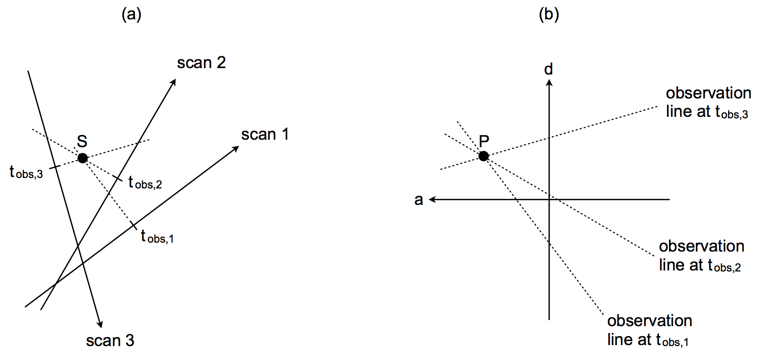
Recall that the geometric instrument model in Equation 4.117 is a parametric description of the ‘observation line’ in field angles $(\eta,\zeta)$ . Let $t_{\text{obs}}$ be the time when the image of a point source crosses this observation line with a known set of indices $f$ , $n$ , $g$ , and $w$ . Using the field index and the known attitude at $t_{\text{obs}}$ , it is possible to calculate the projection of the observation line onto the $(a,\,d)$ plane. In the absence of observational errors the actual point source must obviously be located somewhere along this line in LPC coordinates (Figure 4.16).

The presence of COMA terms in the geometric instrument model complicates this simple picture. The projection of the observation line in LPC is no longer unique, but depends on the assumed colour or the source. This is not a big problem as long as the object consists of a single point source with a known colour: including the COMA terms when computing the projections should still define a unique position. However, we also want to use the LPC for more complex objects, for example a partially resolved binary with components of different colours. We then need to compute the location in $(a,\,d)$ of each observed CCD sample $N_{k}$ (cf. Equation 3.5), using the time $t_{k}$ of the sample and the attitude and calibration data. But which colour should be used for the individual samples, if the calibration has non-zero COMA terms? Because of the overlapping LSF of the two sources, a sample does not uniquely belong to one or the other component, and therefore has no well-defined colour.

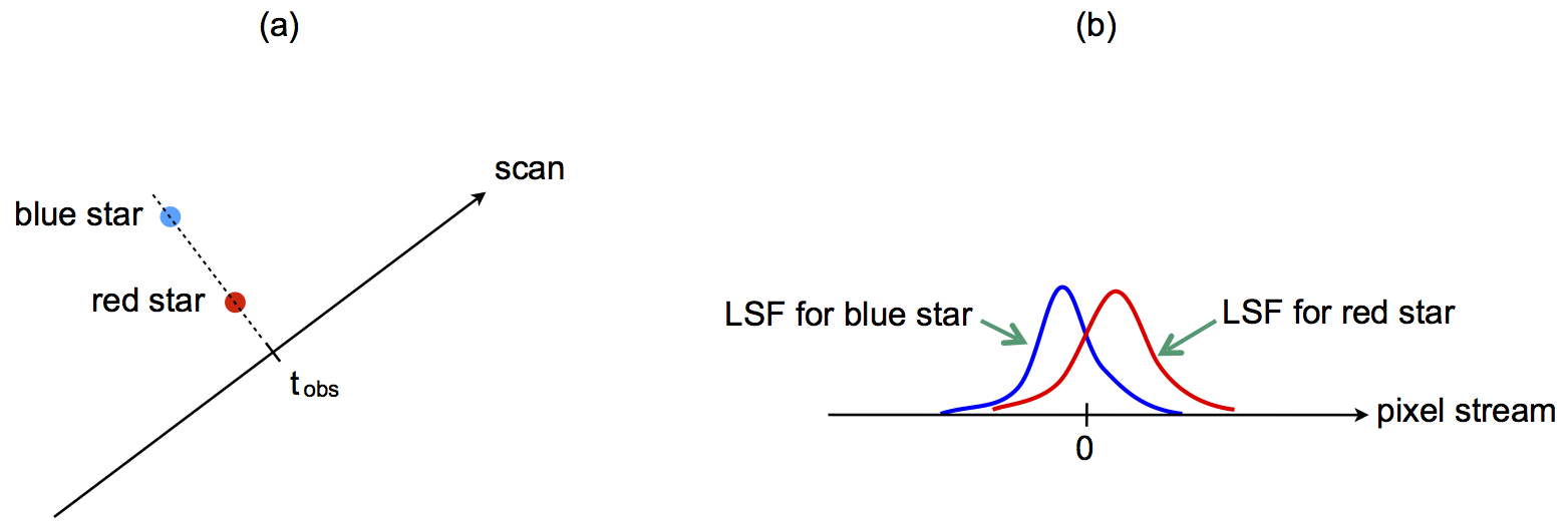
Figure 4.17: Chromaticity and the locations of the images of a blue and red star in the the pixel stream. (a) A binary consisting of a blue and a red star is scanned in a direction perpendicular to the arc connecting the stars. Conceptually, the observation time $t_{\text{obs}}$ should be the same for both components. (b) The image profiles (LSF) generated by the components are different due to the chromaticity of the instrument. However, if the origin of the LSF is achromatic, the two profiles have the same origin ‘0’, and the locations returned by the image parameter determination will also be the same. This will facilitate the analysis of the system in (a).

The conceptually simplest solution to this difficulty is to ensure that the origin of the LSF is achromatic, i.e. independent of colour. The meaning of this is illustrated in Figure 4.17. The chromatic terms in the geometric instrument model should then be strictly zero. Similarly, one must ensure that the origin of the LSF is independent of $G$ , in which case the magnitude-dependent terms of the geometric instrument model are zero.

These conditions were not met in the first two cycles of the Gaia data processing, leading to Gaia DR1 and Gaia DR2, and were only partially met for Gaia EDR3. The geometric instrument model must therefore still include COMA terms that in general are non-zero. In subsequent cycles the COMA terms should eventually vanish as these effects instead become part of the PSF and LSF calibrations. Complete elimination of these effects by means of the PSF/LSF calibration will require several iterations of the cyclic processing loop. Even then, the COMA terms may however be retained in the astrometric solution for diagnostic purposes.

To achieve a colour- and magnitude-independent origin of the calibrated PSF and LSF, one needs the expected location of an image in the absence of COMA effects, precisely in order to include these effects in the PSF/LSF calibration. In the AGIS-PhotPipe-IDU iteration loop (Section 4.4.6), when the calibration parameters from the AGIS solution are fed back to the Intermediate Data Update (IDU), the COMA terms must therefore be set to zero.

gaia early data release 3 documentation

4.3.6 Geometric instrument model

AL geometric instrument model

AC geometric instrument model

Constraints

COMA terms