3.4 Processing steps 3.4.4 Basic angle variation determination 3.4.6 Barycentric radial velocity correction (BVC)

3.4.5 On-ground attitude reconstruction (IOGA, OGA1, OGA2 and SDMOGA)

Author(s): David Hobbs, Michael Biermann, Jordi Portell, Javier Castañeda

The processing of attitude telemetry from the Gaia spacecraft is unique due to the high accuracy requirements of the mission. Normally, for science missions, the on-board measured attitude from the star trackers, in the form of attitude quaternions, would be sufficient for the scientific data reduction but perhaps requiring some degree of smoothing and improvement before use. Such a raw attitude would be accurate to the order of a few arcseconds ( ${}^{\prime\prime}$ ) but for the Gaia mission, an attitude accurate to a few tens of $\mu$ as is required. This is achieved through a series of processing modules and data products as illustrated in Figure 3.12.

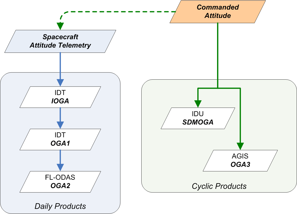
Figure 3.12: Schematic overview of the attitude processing modules and products.

The raw attitude is received in telemetry and stored in the IDTFL database. This is then available for IDT, which first performs the Initial On-Ground Attitude (IOGA) reconstruction, which fits a set of B-spline coefficients to the available telemetry, resulting is an array of B-spline coefficients and the associated knot times (see Section 4.3.5). The output from IOGA can then be used as the input to the first On-Ground Attitude (OGA1) reconstruction, which is a Kalman filter designed to smooth the attitude and to improve its accuracy to the order of 50 mas using a preliminary cross-match infomation against the ASC (see Section 3.2.3). At this point, more Gaia specific processing begins. For Gaia, a First Look (FL) process is employed to do a direct astrometric solution on a single days worth of data, known as the One Day Astrometric Solution (ODAS). This is basically a quality check on the Gaia data but also results in an order of magnitude improvement in the accuracy of the attitude. After ODAS, the attitude is known as OGA2 and is available in the form of B-splines and quaternions. OGA2 is the intended nominal input to other daily downstream system and to AGIS, although it would also be possible to use OGA1 from IDT as input. However, in practice, mainly due to data gaps and discontinuities in the daily processing, it has been found that a simple spline fit to the commanded attitude (see Section 1.3.2) is sufficient for initializing AGIS processing. AGIS is the final step in the attitude improvement, where all the available observations for primary stars are used together with the latest available cross-match, attitude and calibration parameters to iteratively arrive at the final attitude solution. This AGIS final attitude is referred to as the OGA3 (Section 4.3.5). It is worth mentioning that after Gaia DR2, IDU also performs its own attitude refinement, known as SDMOGA, which is needed for the Scene, Detection classifier and cross-match tasks (SDM). The reason is that IDU is the first DPAC system processing all the raw data accumulated during a given data reduction cycle, and therefore, the most recent observations are not covered by OGA3 yet. Although IDU could combine OGA3 with OGA1 or OGA2 for the most recent observations, the decision was to perform a new overall refinement so eventual issues in the daily systems propagated to OGA3 are avoided. Additionally, with SDMOGA the accuracy and precision of the attitude is consistent and uniform throughout the complete time extent.

IOGA

In IDT, the raw attitude values from the AOCS are processed to obtain a mathematical representation of the attitude as a set of spline coefficients. The details of the spline fitting are outlined in Appendix A of Lindegren et al. (2012). The result of this fitting process is the Initial OGA (IOGA). The time intervals processed can be defined by natural boundaries, like interruptions in the observations, e.g., due to micro-meteorites. The boundaries can also be defined by practical circumstances, like the end of a data transmission contact, or the need to start processing.

Using IOGA, a list of sources is extracted from the Attitude Star Catalogue (ASC; Section 3.2.3) in the bands covered by Gaia during the time interval being processed. In the early phases of the mission (for Gaia DR1), the ASC was a subset of the IGSL, but in Gaia DR2, the ASC has been replaced by stars from the MDB catalogue. This allows the next process, OGA1, to run efficiently, knowing in advance if a given observation is likely to belong to an ASC star.

OGA1

The main objective of OGA1 is to reconstruct the non-real-time First On-Ground Attitude (OGA1) for the Gaia mission with high accuracy for further processing. The accuracy requirements for the OGA1 determination (along and across scan) are 50 mas (to be improved later on in the mission to 5 mas). OGA1 relies on an Extended Kalman filter (EKF) to estimate the orientation, $\mathbf{q}$ , and angular velocity, $\boldsymbol{\omega}$ , of the spacecraft with respect to the Satellite Reference System (SRS), defining the state vector

\boldsymbol{x}=\left(\begin{matrix}\mathbf{q}\\ \boldsymbol{\omega}\end{matrix}\right)\,.

(3.14)

System model

The system model is fully described by two sets of differential equations, the first one describing the satellite’s attitude following the quaternion representation

\mathbf{\dot{q}}(t)=\frac{1}{2}\boldsymbol{\Omega}({\boldsymbol{\omega}})% \mathbf{q}(t),

(3.15)

where

\boldsymbol{\Omega}({\boldsymbol{\omega}})=\begin{bmatrix}0&\omega_{z}&-\omega% _{y}&\omega_{x}\\ -\omega_{z}&0&\omega_{x}&\omega_{y}\\ \omega_{y}&-\omega_{x}&0&\omega_{z}\\ -\omega_{x}&-\omega_{y}&-\omega_{z}&0\\ \end{bmatrix},

(3.16)

and the second one using the Euler’s equations:

\dot{\boldsymbol{\omega}}(t)=I_{\rm sc}^{-1}(T_{\rm e}-\boldsymbol{\omega}% \times I_{\rm sc}\boldsymbol{\omega}),

(3.17)

where $I_{\rm sc}$ is the moment of inertia of the satellite and $T_{\rm e}$ is the total of disturbance and control torques acting on the spacecraft. The satellite is assumed to be represented as a freely rotating rigid body, which implies to set the external torques to zero in Equation 3.17. If this simplification does not work well when reconstructing the Gaia attitude then the proper $T_{\rm e}$ , including external torques, that is required to follow the NSL should be taken into account.

Process and measurement model

The process model predicts the evolution of the state vector $\boldsymbol{x}$ and describes the influence of a random variable $\mu(t)$ , the process noise. For non-linear systems, the process dynamics is described as follows:

\dot{\boldsymbol{x}}(t)=\boldsymbol{f}(\boldsymbol{x}(t),t)+\boldsymbol{G}(% \boldsymbol{x}(t),t)~{}\mu(t),

(3.18)

where $\boldsymbol{f}$ and $\boldsymbol{G}$ are functions defining the system properties. For OGA1, $\boldsymbol{f}$ is given by Equation 3.15 and Equation 3.17, and $\mu(t)$ is a discrete Gaussian white noise process with variance matrix $\boldsymbol{Q}(t)$ :

\mu(t)\sim M(0,\boldsymbol{Q}(t))\,.

(3.19)

The measurement model relates the measurement value $\boldsymbol{y}$ to the value of the state vector $\boldsymbol{x}$ and describes also the influence of a random variable $\nu(t)$ , the measurement noise of the measured value. The generalized form of the model equation is:

\boldsymbol{y}_{k}=\boldsymbol{h}(\boldsymbol{x}(t_{k}),t)+\nu(t)

(3.20)

where $\boldsymbol{h}$ is the function defining the measurement principle, and $\nu(t)$ is a discrete Gaussian white noise process with variance matrix $\boldsymbol{R}(t)$ (with standard deviations of 0.1 mas and 0.5 mas along and across scan respectively):

\nu(t)\sim N(0,\boldsymbol{R}(t))\,.

(3.21)

In order to estimate the state, the equations expressing the two models must be linearized in order to use the KF model equations, around the current estimation ( $\boldsymbol{x}^{-}_{k}$ ) for propagation periods and update events.

This procedure yields the following two matrices to be the Jacobian of the $\boldsymbol{f}$ and $\boldsymbol{h}$ functions with respect to the state:

\boldsymbol{F}=\left.\frac{\partial\boldsymbol{f}(\boldsymbol{x}(t),t)}{% \partial\boldsymbol{x}(t)}\right|_{\boldsymbol{x}=\boldsymbol{x}^{-}_{k}}

(3.22)

and

\boldsymbol{H_{k}}=\left.\frac{\partial\boldsymbol{h}(\boldsymbol{x}(t),t)}{% \partial\boldsymbol{x}(t_{k})}\right|_{\boldsymbol{x}=\boldsymbol{x}^{-}_{k}}\,.

(3.23)

KF propagation equations

The KF propagation equations consist of two parts: the state system model and the state covariance equations. The first one,

\dot{\boldsymbol{x}}(t)=\boldsymbol{F}(t)\boldsymbol{x}(t)+\boldsymbol{G}(t)% \mu(t),

(3.24)

can be propagated using a numerical integrator, such as the fourth-order Runge-Kutta method. The $\boldsymbol{F}$ matrix is called the transition matrix, $\boldsymbol{Q}$ the system noise covariance matrix, and $\boldsymbol{G}$ the system noise covariance coupling matrix.

The transition matrix can be expressed as:

\boldsymbol{F}=\begin{bmatrix}0.5\boldsymbol{\Omega}(\boldsymbol{\omega})&0.5% \boldsymbol{\Theta}(\mathbf{q})\\ 0_{3\times 4}&\boldsymbol{F}_{\dot{\boldsymbol{\omega}}\boldsymbol{\omega}}\\ \end{bmatrix},

(3.25)

where

\boldsymbol{\Theta}({\mathbf{q}})=\begin{bmatrix}q_{w}&-q_{z}&q_{y}\\ q_{z}&q_{w}&-q_{x}\\ -q_{y}&q_{x}&q_{w}\\ -q_{x}&-q_{y}&-q_{z}\\ \end{bmatrix},

(3.26)

and

\boldsymbol{F}_{\dot{\boldsymbol{\omega}}\boldsymbol{\omega}}=-\left(I_{\rm sc% }^{-1}([\boldsymbol{\omega\times}]I_{\rm sc}-[(I_{\rm sc}\boldsymbol{\omega})% \times])\right)\,.

(3.27)

Here, the matrix notation $[\boldsymbol{a}\times]$ represents the skew symmetric matrix of the generic vector $\boldsymbol{a}$ . For the state covariance propagation, the Riccati formulation is used:

\dot{\boldsymbol{P}}=\boldsymbol{F}\boldsymbol{P}+\boldsymbol{P}\boldsymbol{F}% ^{T}+\boldsymbol{G}\boldsymbol{Q}\boldsymbol{G}^{T}\,.

(3.28)

Its prediction can be carried out through the application of the fundamental matrix $\boldsymbol{\Phi}$ (i.e., first order approximation using the Taylor series) about $\boldsymbol{F}$ , which becomes:

\boldsymbol{\Phi}(\Delta t)\approx\boldsymbol{I}+\boldsymbol{F}\cdot\Delta t,

(3.29)

where $\Delta t$ represents the propagation step. The process noise matrix $\boldsymbol{Q}$ used for the Riccati propagation Equation 3.28 is considered to be

\boldsymbol{G}\boldsymbol{Q}\boldsymbol{G}^{T}={\rm diag\left(\left[(10^{-8})^% {2},(10^{-8})^{2},(10^{-8})^{2},(10^{-8})^{2},(10^{-8})^{2},(10^{-8})^{2},(10^% {-8})^{2}\right]\right)}

(3.30)

since OGA1 depends more on the measurements (even if not so accurate at this stage) than on the system dynamic model.

KF update equations

The KF update equations correct the state and the covariance estimates with the measurements coming from the satellite. In fact, the measurement vector $\boldsymbol{y}_{k}$ consists of the so-called measured along-scan angle $\eta_{m}$ , and the measured across-scan angle $\zeta_{m}$ , and they are the values as read from the AF1 CCDs.

On the other hand, the calculated field angles ( $\boldsymbol{h}(\boldsymbol{x}_{t})=[\eta_{c},\zeta_{c}]$ ) are the field angles calculated from an ASC for each time of observation. The set of the update equations are listed below:

	$\displaystyle\hat{\boldsymbol{x}}^{+}_{k}=\hat{\boldsymbol{x}}^{-}_{k}+% \boldsymbol{K}_{k}\left[\boldsymbol{y}_{k}-\boldsymbol{h}_{k}(\hat{\boldsymbol% {x}}^{-}_{k})\right],$		(3.31)
	$\displaystyle\boldsymbol{P}^{+}_{k}=\left[\boldsymbol{I}-\boldsymbol{K}_{k}% \boldsymbol{H}_{k}(\hat{\boldsymbol{x}}^{-}_{k})\right]\boldsymbol{P}_{k}^{-},$		(3.32)
	$\displaystyle\boldsymbol{K}^{+}_{k}=\boldsymbol{P}_{k}^{-}\boldsymbol{H}_{k}^{% T}\left[\boldsymbol{H}_{k}\boldsymbol{P}_{k}^{-}\boldsymbol{H}_{k}^{T}+% \boldsymbol{R}_{k}\right]^{-1},$		(3.33)

where the measurement sensitivity matrix $\boldsymbol{H}_{k}$ is given by:

\boldsymbol{H}_{k}=\begin{bmatrix}\frac{\partial\eta_{k}}{\partial\mathbf{q}}&% 0_{1\times 3}\\ \frac{\partial\zeta_{k}}{\partial\mathbf{q}}&0_{1\times 3}\end{bmatrix},

(3.34)

and the measurement noise matrix $\boldsymbol{R}$ is chosen such that:

\boldsymbol{R}=\begin{bmatrix}\sigma_{\eta}^{2}&0\\ 0&\sigma_{\zeta}^{2}\\ \end{bmatrix}.

(3.35)

The standard deviation for the field angle errors along and across scan are computed and provided by IDT.

The processing scheme

The OGA1 process can be divided in three main parts: input, processing, and output.

The inputs are:

•
Oga1Observations (OGA1 needs these in time sequence from IDT) composed essentially by:
- –
  
  transit identifiers (TransitId)
- –
  
  observation times (TObs)
- –
  
  observed field angles (FAs) including geometry calibration
•

A raw attitude (IOGA), with about 7 ${}^{\prime\prime}$ noise (in B-splines).
•

A cross-match table with SourceId–TransitId pairs plus a proper direction to the star at the instance of observation.

The OGA1 determination is a Kalman Filter (KF) process, i.e., essentially an optimization loop over the individual observations, concluded by a spline-fitting of the resulting quaternions. The main processing steps are:

•

Sort the list of elementaries by time. Then sort the list of cross-match sources by the transit identifier with the ones from the sorted list of elementary. The unmatched elementary transits are simply discarded.
•

Initialize the KF: interpolate the B-spline (IOGA attitude format) in order to get the first quaternion and angular velocity to start the filter. Optionally, the external torque can be reconstructed in order to have a better accuracy for the dynamical system model.
•

Forward KF: for a generic time $t_{i}$ , predicting the attitude quaternion from the state vector at the time $t_{i-1}$ of the preceding observation.
•

Backward KF: for a generic time $t_{i-1}$ , predicting the attitude quaternion from the state vector at the time $t_{i}$ of the preceding observation. Backward propagation is needed to reduce errors near the start of the time interval.
•

Compute the field coordinates from the pixel coordinates for SM and AF measurements, using a Gaia calibration file. OGA1 uses the AF2 values as observed field angles.
•

Compute field coordinates of known stars (from the ASC).
•

Correct the state using the difference between the observed and the calculated measurements in the along-scan ( $\Delta\eta$ ) and across-scan ( $\Delta\zeta$ ) directions.
•

Generate a B-spline representation for the whole time interval at the end of the loop over the measurements.
•

Remove any attitude spike that may appear, for example due to a wrong cross-match record.

The outputs are the improved attitude (for each observation time $t_{i}$ ) in two formats:

•

Quaternions $\mathbf{q}_{OGA1}(t_{i})$ in the form of arrays of doubles.
•

A B-spline representation from the OGA1 quaternions.

The OGA1 process, being a Kalman filter, needs its measurements in strict time sequence. In order to keep the OGA1 process simple, the baseline is to separately use the CCD transits. OGA1 relies on two-dimensional (2D) astrometric measurements from Gaia. That is, CCD transits of stars used by OGA1 must have produced 2D windows. OGA1 furthermore requires at least about one such 2D measurement per second and per FoV, in order to obtain the required precision.

OGA2 and ODAS source positions

The main objective of the ODAS (see Section 3.5.2) is to produce a daily, high-precision astrometric solution that is analysed by First Look Scientists in order to judge Gaia’s instrument health and scientific data quality (see also Section 3.5.2). The resulting attitude reconstruction, OGA2, together with source position updates computed in the framework of the First Look system, is also used as input parameter by the Daily spectroscopic wavelength calibration. For the first two data segments (Table 1.7), OGA2 was accurate to the 50 mas level because it was (like OGA1) tied to the reference system of the ground-based ASC. After switching to the Gaia DR2 based reference system, the OGA2 for the third data segment is accurate to the 5-mas level. For all data segments the OGA2 is, however, precise at the sub-mas level, i.e., internally consistent, except for a global rotation with respect to the ICRF.

The computation of OGA2 is not a separate task but one of the outputs of the ODAS (One-Day Astrometric Solution) software of the First Look System (see Section 3.5.2). This process can be divided into three main parts: input, processing, and output:

1.
The OGA2 inputs are outputs of the IDT system, namely:
- –
  
  AstroElementaries with transit IDs and observation times,
- –
  
  OGA1 quaternions $\mathbf{q}_{OGA1}(t_{i})$ ,
- –
  
  a source catalogue with source IDs, and
- –
  
  a cross-match table with pairs of source IDs and transit IDs.
2.

The processing steps: the OGA2 attitude is determined in one go together with daily geometric instrument calibration parameter updates and updated source positions in the framework of the First Look ODAS system (which is a weighted least-square method).
3.

The OGA2 output is a B-spline representation of the improved attitude (as a function of observation time $t_{i}$ ).

Along with OGA2, First Look produces on a daily basis improved sources positions which also are used as input parameters by the Daily photometric and spectroscopic wavelength calibrations for the more recent data received from the spacecraft. The accuracy and precision levels of the source positions are the same as those of OGA2.

SDMOGA

The need of a new attitude refinement for the cyclic processing in IDU was first identified in Gaia DR1 to be able to recover the attitude gaps from the Daily pipeline (OGA1 from IDT and OGA2 from FL) which were persisted in the DRC processing (OGA3 in AGIS). Additionally, SDMOGA is more robust and stable as it runs over a more complete and consolidated set of inputs and contrary to the daily processing approach, this implementation does not pursue a near-real-time processing and therefore can benefit of the already known events on the satellite.

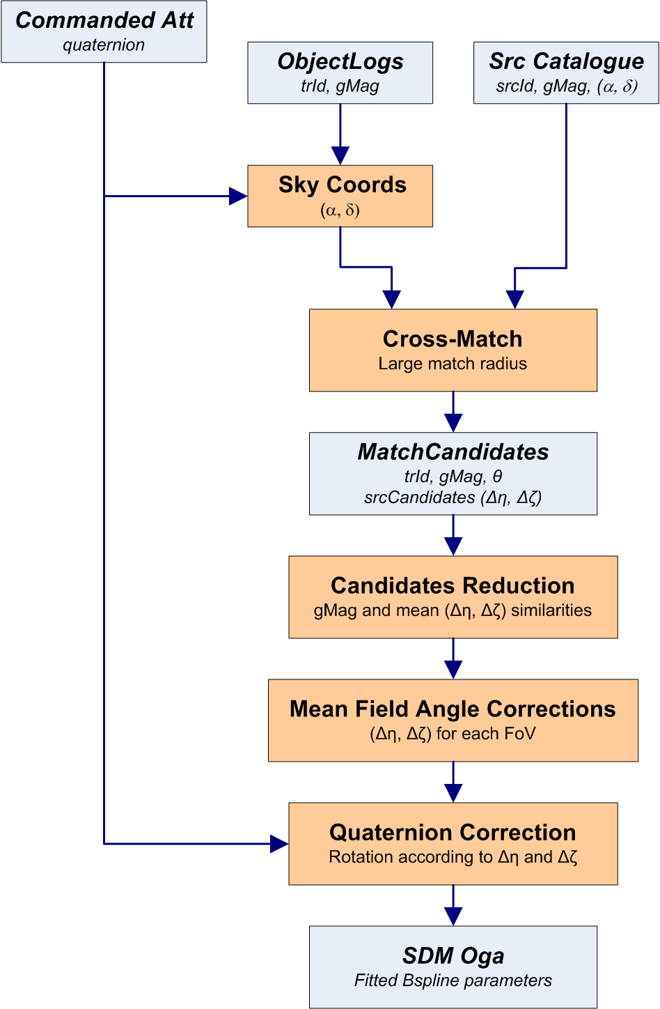
SDMOGA processing is split in time intervals that run in parallel as separated jobs, each job load data from the preceding and following time intervals to assure the continuity of the fitting in the time interval edges. Every job performs the following processes (see Figure 3.13):

1.

Compute sky coordinates for all the loaded observations using the commanded attitude (see Section 1.3.2).
2.

Perform a cross-match against a reference source catalogue (see Section 3.2.3) using a large matching radius of the order of 40 arcsec to account for the low accuracy of the spacecraft following the commanded attitude.
3.

Process the source candidates for each observation reducing the ambiguitiy according to the magnitude similarity and the observation-source distance. The sources candidates are filtered by distance according to a user-defined thresholds centered in the trimmed mean of the observed distances of all source candidates using an sliding time window of few seconds. After this step only observations with only one source candidate survive.
4.

Process the distance measurements of the surviving observation-source pairs computing the corrections to be applied to the original commanded attitude quaternions. These corrections are again computed as the trimmed mean of the distances of the surviving observation-source pairs using another sliding time window of few seconds.
5.

Fit a B-Spline over the corrected quaternions generating the SDMOGA record (see Section 4.3.5). In general only one SDMOGA record is generated in each job but additional records may be produced in case of major time gaps.

Figure 3.13: Schematic overview of the SDMOGA attitude processing.

SDMOGA attitude is accurate to the 5-mas level and precise at the sub-mas level (similar to the more recent OGA1 and OGA2 solutions).

gaia early data release 3 documentation