3.3.3 CCD health, charge injection and release

Author(s): Michael Davidson

The focal plane of Gaia contains 106 CCDs, each with 4494 lines and 1966 light-sensitive columns, leading to it being called the ‘billion pixel camera’. The pre-processing requires calibrations for the majority of these CCDs, including SM, AF, and BP/RP, in order to model each window during image parameter determination. Where effects cannot be adequately modelled, the affected CCD samples can be masked and the observations flagged accordingly. The CCDs are affected by the kind of issues familiar from other instruments such as dark current, pixel non-uniformity, non-linearity, and saturation (see Janesick 2001). However, due to the operating principles used by Gaia such as TDI, gating, and source windowing, the standard calibration techniques need sometimes to be adapted. The use of gating generally demands multiple calibrations of an effect for each CCD. In essence, each of the gate configurations must be calibrated as a separate instrument.

The various effects must be monitored and the calibrations redetermined on an on-going basis to identify changes, for instance the appearance of new defects such as hot columns. To minimise disruption of normal spacecraft operations, most of the calibrations must be determined from routine science observations. Only a few calibrations demand a special mode of operation, such as ‘offset non-uniformities’ and serial-CTI measurement (e.g., Section 1.3.4, Section 1.3.4, Section 3.3.2, and Fabricius et al. 2016). There are two main data streams used in this calibration: 2D science windows and Virtual Objects (VOs; Section 1.1.3). The 2D science windows typically contain bright stars, although a small fraction of faint stars which would otherwise be assigned a 1D window are acquired as 2D (known as Calibration Faint Stars, CFSs). VOs are ‘empty’ windows which are interleaved with the detected objects, when on-board resources permit. By design, the VOs are placed according to a fixed repeating pattern which covers all light-sensitive columns every two hours, ensuring a steady stream of information on the CCD health. The VOs allow monitoring of the faint end of the CCD response while the 2D science windows allow us to probe the bright end.

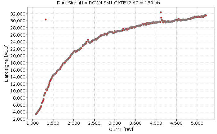
Dark signal (or dark current) is the charge produced by each column of a CCD when it is in complete darkness. While such a condition was achieved during the on-ground testing, it is not possible to replicate in flight as there are no shutters on Gaia. The observed VO windows must therefore be used to determine the dark signal, although these also contain background, source and contamination signal, bias non-uniformity, and CTI effects. An independent library is produced every 10 revolutions. Eligible input observations are selected, for instance those not containing multiple gates or charge injections. The electronic bias (including non-uniformity) is subtracted from each window and a source mask is created via an N-sigma clipping of the de-biased samples. The leading samples in the window are also masked to mitigate CTI effects. A least-squares method is then used to estimate a local background for the window (assumed to be uniform), and this in turn can be subtracted to provide a measure of the dark signal in each CCD column covered by the window. In this manner, measures can be accumulated for each column over the 10 revolution interval, and then a median taken (with a positivity constraint) to provide a robust dark signal value. There are two notable limitations in the modelling. Firstly, sub-optimal bias non-uniformity correction can produce column-level artefacts, leading to a relatively high threshold for hot-column masking of 5 ADU. The strongest defects are well-tracked as seen in the example in Figure 3.5. Secondly, VO data are ungated in AF so cannot provide information on the dark signal over the short gates. We apply a linear scaling of the NOGATE level although this does not generally reflect the step-change behaviour expected due to the presence of hot pixels.

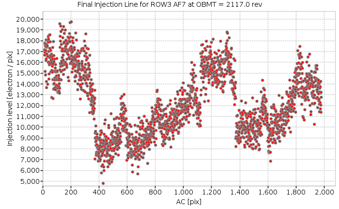
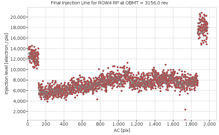
To mitigate the effect of CTI there are periodic lines of injected charge; four consecutive lines every 2000 TDI1 or 5000 TDI1 in AF and XP respectively. These charge packets fill any available traps and so the change in observed injection level between each line provides valuable information on the damage level. The injections also have very significant and variable (between devices) across-scan profile. It is therefore necessary to calibrate the injections at pixel-resolution using VOs and faint CFS science windows. Since we now know that the injection levels are extremely stable a long interval can be used to accumulate data for each calibration. The bias and dark signal are subtracted and a background determined for each window in order to obtain measures of the injection level at each line and column, which in turn are used to compute a robust median level. In Gaia EDR3 we use an interval of approximately 1039 revolutions to produce four independent libraries. The calibrated levels are seen to be stable in time with a typical variation of only 0.01%. As seen in Figure 3.6 the level can vary significantly between columns plus there are a few tens of discrete column defects over the AF/XP devices caused by deep traps, injection structure anomalies and anti-blooming drain issues.

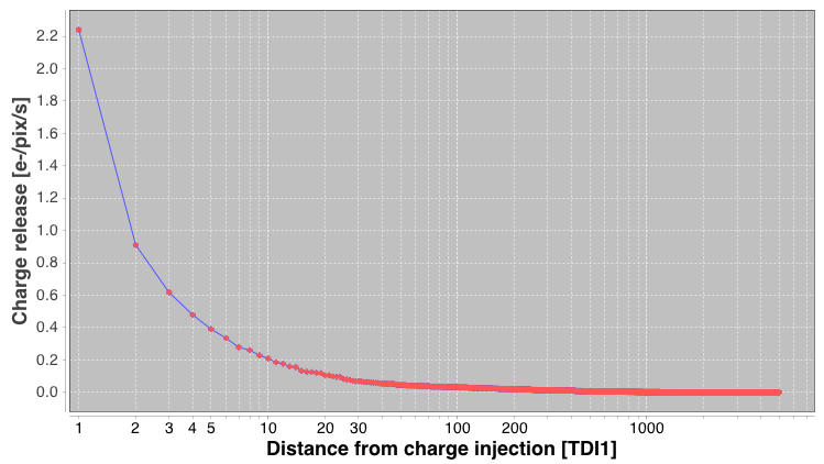
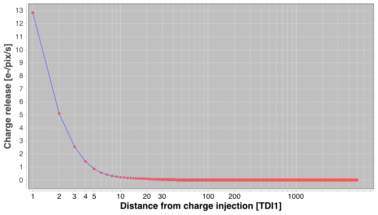
The injected charge which has filled traps is subsequently released on time-scales related primarily to the species of trap defect. Rather than attempt an analytical model such as a sum-of-exponentials to represent these charge release trials following injections we instead calibrate the profile as a look-up table at full TDI1 resolution. Virtual objects and faint science windows are used to obtain measures of the release profile by subtracting the bias and dark signal and fitting a background per window. A single release profile is found for each device, which is then scaled by the injection level at each column. For robustness the profile is constrained to be positive and monotonically decreasing with distance from the injection. By convention the end of the release trail is defined to have a value of zero; it is never possible to fully separate the contribution of the charge release from other background sources. Examples of some charge release profiles are seen in Figure 3.7.

In an ideal device, there would be a linear response between the accumulated charge and the output of the Analogue-to-Digital Converters (ADCs) at all signal levels. In reality, the response typically becomes non-linear at high input signals for a variety of reasons (see Janesick 2001). Although the linearity has been measured before launch, a calibration was not yet implemented in the processing pipeline due to the uncertainty in determination of the input signals, which require detailed knowledge of a range of coupled CCD effects. In the meantime, a conservative linearity threshold has been used to allow masking of samples which may be within the non-linear regime. A related topic is the pixel non-uniformity which represents the variation in sensitivity across the CCD. In Gaia, we observe only the integrated sensitivity of the pixels within a particular gate so this is known as the Column Response Non-Uniformity (CRNU). Similarly, no in-flight calibration had yet been performed apart from the extreme case to identify ‘dead’ columns. These are columns which appear to have zero sensitivity to illumination and can be found using bright-star windows. The accumulated samples for a dead column have a distribution which is consistent with the expected dark signal plus readout noise. The CCDs used on Gaia have been selected for their excellent cosmetic quality (see also Section 1.3.4).

At the highest signal levels, various saturation effects occur on the device and within the ADC. There can be large differences in the effective saturation level across a single device, or even between neighbouring columns, for example due to variation in the Full Well Capacity (FWC). For reasons beyond the scope of this document, the saturation level can oscillate or jump depending on the readout sequencing. An algorithm has been developed to measure the lowest observed saturation level for each gate and column to allow conservative masking of samples. A Mexican hat filter is applied to the accumulation of samples from bright-star windows to identify over-densities of data at particular signal levels, using analytical significance thresholds. The lowest significant peak is then taken as the saturation level. If no peak is found, then the maximum observed sample for that column is used.