3.3.2 CCD bias and non-uniformity
Author(s): Nigel Hambly
As is usual in imaging systems that employ charge-coupled devices (CCDs) and analogue-to-digital converters (ADCs), the input to the initial amplification stage of the latter is offset by a small, constant voltage to prevent thermal noise at low signal levels from causing wrap-around across zero digitised units. The Gaia CCDs and associated electronic controllers and amplifiers are described in detail in Kohley et al. (2012). The readout registers of each Gaia CCD incorporate 14 prescan pixels (i.e., those having no corresponding columns of pixels in the main light-sensitive array; Figure 1.4). These enable monitoring of the prescan levels, and the video chain noise fluctuations for zero photo-electric signal, at a configurable frequency and for configurable across-scan (AC) hardware sampling. In practice, the acquisition of prescan data is limited to the standard un-binned (1 pixel AC) and fully binned (2, 10, or 12 pixel AC depending on instrument and mode) and to a burst of 1024 one-millisecond samples each once every 70 minutes in order that the volume of prescan data handled on board and telemetred to the ground does not impact significantly on the science data telemetry budget.
Video chain offset levels and total detection noise
The read noise (or, more correctly, the video chain total detection noise including noise contributions from CCD readout noise, ADC and quantisation noise, etc.) can be assessed from the short timescale fluctuations measured in the prescan levels. Figure 3.1 shows the offset levels and measured total detection noise for the FPA science devices. Table 3.1 gives a summary of the required and measured noise properties of the various instrument video chains. From the sample-to-sample fluctuations measured in the 1 second prescan bursts, all devices are operating well within the requirements. All devices are operating nominally as regards their offset and read noise properties.
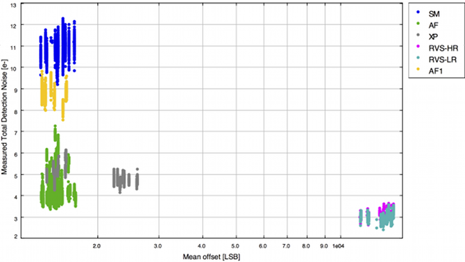
| Instrument | Mean gain | Total detection noise per sample | ||
| and mode | ADU / e | Required / e | Measured / e | Measured / ADU |
| SM | 0.2569 | 13.0 | ||
| AF1 | 0.2583 | 10.0 | ||
| AF2–9 | 0.2578 | 6.5 | ||
| BP | 0.2464 | 6.5 | ||
| RP | 0.2484 | 6.5 | ||
| RVS–HR | 1.7700 | 6.0 | ||
| RVS–LR | 1.8185 | 4.0 | ||
Offset stability
The approximately hourly monitoring of the prescan pixels is suitable for characterising any longer timescale drifts in the offsets characteristics. For example, Figure 3.2 shows the total video chain detection noise as measured from prescan fluctuations over an extended period of over 1000 revolutions (corresponding to more than 250 days). Over this period (July 2014 to May 2015) there is no discernible degradation in the video chain performance. This remains true up to the day of writing (Summer 2020).
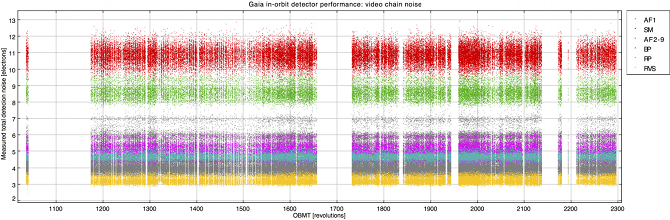
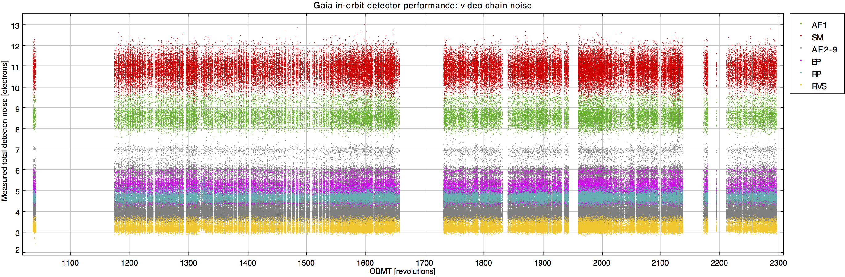
Figure 3.3 shows the long timescale stability of one device in the Gaia focal plane. In this case (device AF2 on row 4 of the FPA), the long term drift over more than 100 days is ADU, apart from the electronic disturbance near OBMT revolution 1320 (this was caused by payload module heaters being activated during a ‘de-contamination’ period in September 2014; Table 1.10). The roughly hourly monitoring of the offsets via the prescan data allows the calibration of the additive signal bias early in the daily processing chain, including the effects of long timescale drift and any electronic disturbances of the kind illustrated in Figure 3.3. The ground segment receives the bursts of prescan data for all devices and distils them into ‘bias records’ containing one or more bursts per device. These provide robustly estimated mean levels along with dispersion statistics for noise performance monitoring. Spline interpolation amongst these values is used to provide an offset model at arbitrary times within a processing period. Figure 3.4 shows a detailed example around the large excursion seen in Figure 3.3.
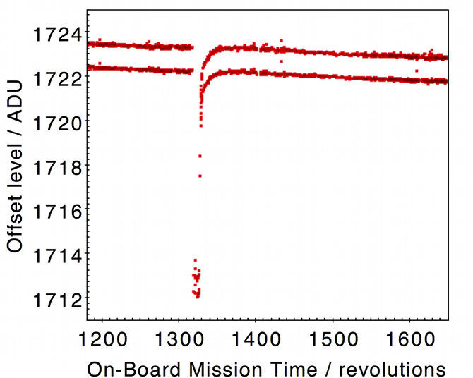
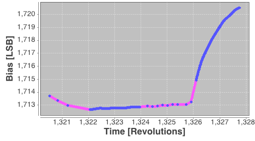
Figure 3.3 illustrates the small offset difference between the un-binned and fully binned sample modes for the device in question. In fact, there are various subtle features in the behaviour of the offsets for each Gaia CCD associated with the operational mode and electronic environment. These manifest themselves as small (typically a few ADU for non-RVS video chains, but up to 100 ADU in the worst-case RVS devices), very short timescale (10 s) perturbations to the otherwise highly stable offsets. The features are known collectively as ‘offset non-uniformities’ and, because the effect presumably originates somewhere in the CCD–PEM coupling, it is also known as the ‘PEM–CCD offset anomaly’. The effect requires a separate calibration process and a correction procedure that involves the on-ground reconstruction of the readout timing of every sample read by the CCDs since they are a complex function of the sample readout sequencing. For a detailed description of the characteristics of these non-uniformities along with their calibration and correction, see Hambly et al. (2018b).