4.5.5 Geometric calibration verification
Author(s): Alex Bombrun
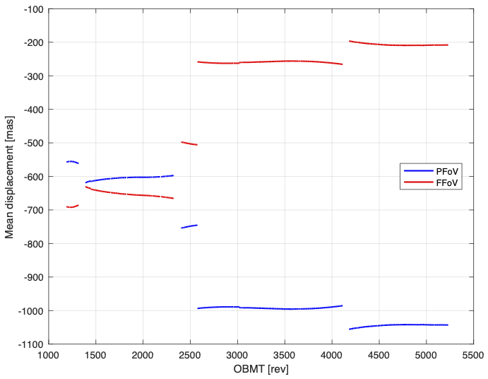
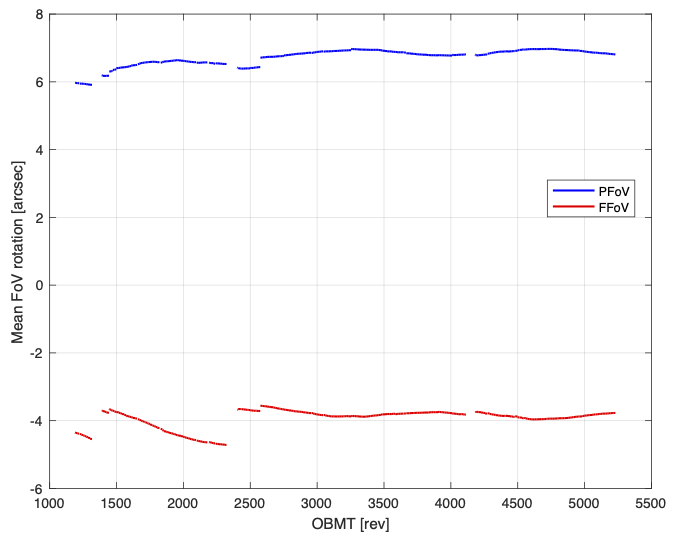
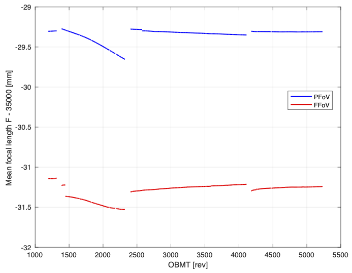
The calibration model is described in Section 4.3.6. This model is more complex than the original proposal to take into account effects not corrected yet in the PSF/LSF calibration Section 3.3.5. The validation of the calibration model is strongly tied to the analysis of AGIS residuals, i.e. one looks for any dependencies in the residuals that can be compensated by some effect in the calibration model. Besides the analysis of the residuals one can also plot the calibration parameters and check that they are consistent with the instrument history. An example of this is given in Figure 4.24.
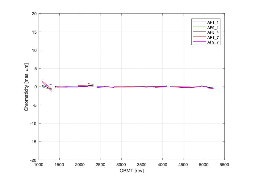
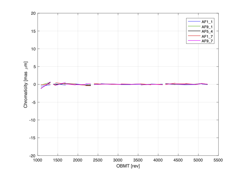
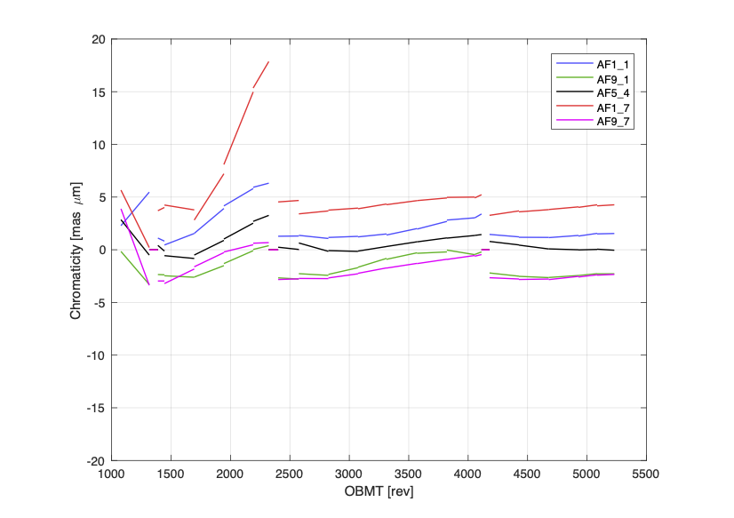
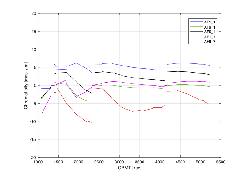
In particular the calibration model contains chromatic corrections (see Section 4.3.4) that were critical to get a good astrometric solution. In Figure 4.25 and Figure 4.26 one can see the time evolution of the chromatic corrections for selected CCDs and per field of view as computed in AGIS for window class 1 observations. The first figure is for the sources where the available colour information could be used to select the appropriate LSF or PSF to fit in the image parameter determination stage of the pre-processing; the second figure is for the sources without such colour information, where a default colour was assumed for the image parameter determination. Comparison of the two figures shows that the colour-dependent LSF/PSF calibration in IDU, based on an earlier AGIS solution, successfully eliminated most of the chromaticity, thus demonstrating the validity of the AGIS-PhotPipe-IDU loop processing described in Section 4.4.6.
Besides residual analysis and plotting of the fitted calibration values, one can also compare the geometric calibration model to the BAM metrology. In particular, as we have introduced break points in the calibration model corresponding to the times of some of the largest BAM jumps, one can compare the jumps derived from the calibration model with the ones introduced in the basic angle corrector. From the current state of this analysis, it seems that a relatively large fraction of the BAM jumps are not astrometric jumps as they are fully compensated by a jump of opposite amplitude in the calibration model.