8.3.7 Spectrophotometry processing
Author(s): Laurent Galluccio, Marco Delbó, Alberto Cellino, Francesca De Angeli
In Gaia DR3, reflectance spectra in visible light for SSOs were computed. These are, essentially, numbered asteroids observed during Cycles 1-3 of the mission.
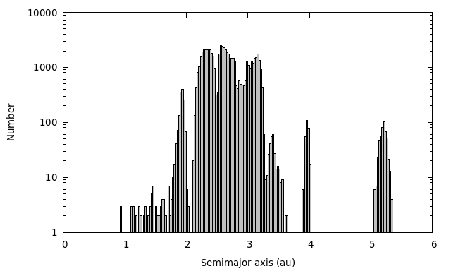
Whereas most of these SSOs reside in the main belt, the near-Earth, Hungaria, Hilda, and Jupiter Trojan populations were also sampled (Figure 8.12).
Each SSO was observed at multiple epochs. Each epoch corresponds to an SSO transit on the Gaia focal plane. For each epoch, internally calibrated BP and RP spectra were extracted (Chapter 5.4.1). Following classical methods (Bus and Binzel 2002), asteroid epoch reflectance spectra were computed by dividing, at each wavelength, the epoch spectrum by an average of mean spectra of a number of solar analogue stars (Section 8.3.7). An epoch spectrum corresponds to a single observation of an object crossing the focal plane. The internal calibration process does not attempt any re-sampling or fitting of the 60 sample measurements that normally constitute an epoch spectrum. Each sample is assigned a pseudo-wavelength value and a flux in the internal reference system. Epoch spectra are not included in Gaia DR3. Mean spectra instead include information from several observations of the same object. In this case, the resulting spectrum is a continuous function defined as a combination of basis functions. See Section 5.3 and Carrasco et al. (2021) for more details.
Next, the obtained epoch spectral reflectances were converted into discrete wavelength channels in the interval from to nm (Section 8.3.7). The final validation of the spectra is described in Section 8.4.5.
Solar analogue stars
Solar analogues, also referred to as solar twins, are stars having physical properties (e.g., mass, metallicity, temperature, age) close to those of the Sun. For the purposes of computation of asteroid spectral reflectances, however, solar analogues are stars whose spectra are similar to that of the Sun. This means that reddened solar twins are not suitable to be used as solar analogue stars. Solar analogue stars serve as calibrators in order to reveal how an asteroid’s surface reflects incoming sunlight as a function of wavelength, providing information about the surface mineralogy.
In ground-based observations, typically, a single solar analogue star close to the asteroid on the sky plane is selected for spectral calibration. Alternatively, two stars are also used in some cases, namely, one star located at no more than few degrees away from the asteroid and having a spectral class G2V or similar is used for telluric correction, while the other ’trusted’ solar analogue that can be located at different air mass is also used to correct for the residual slope induced by the first star in the asteroid’s spectral reflectance.
Given the temporal stability of the Gaia instruments and the fact that the observations are carried out outside the Earth’s atmosphere, it was decided to adopt a method that is believed to be better in principle, being based on the idea of dividing each asteroid’s spectrum by that of the average spectrum of a series of trusted solar analogue stars. This tends to smooth out any noise due to the unavoidable small differences among different solar analogue stars. In detail, the following procedure was developed, based on two steps:
-
•
A list of solar analogue stars was created based on research of most frequently used solar analogues for asteroid spectroscopy in the literature (Table 8.6).
-
•
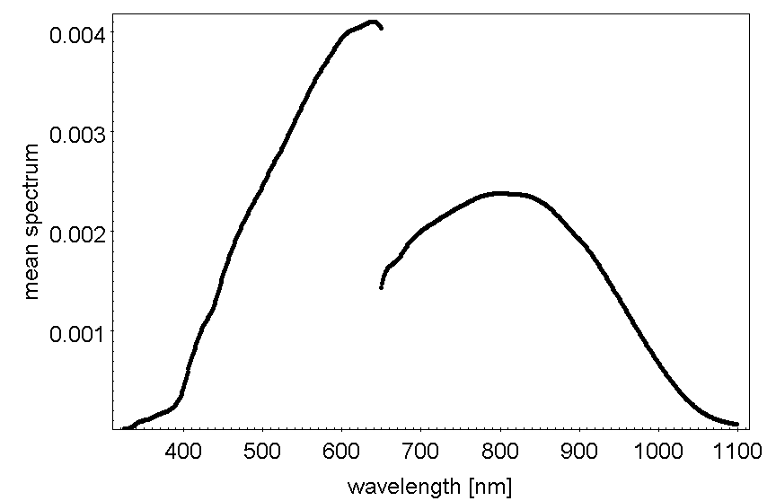
An average spectrum was computed from all the spectra in the list. First, each spectrum was normalised by dividing, point by point, by the sum of the and fluxes and, then, the average spectrum of all normalised spectra and its uncertainty were computed (Figure 8.13).
Following the analysis of the mean spectra, little variations across the sample were found. A subset of these stars spectroscopically closest to each other was extracted. Table 8.6 presents the list of the solar analogue stars selected to compute the mean spectra. The information relative to the mean computed solar analogue spectrum is available through an auxiliary table which contains the mean flux, corresponding wavelengths, and all Gaia DR3 sourceIds of the stars used.
| Denomination | Gaia DR3 sourceId | RA [] | DEC [] | Spec. Type | Ref. | |
| HD6400 | 2352876238295485440 | 16.178114 | -20.987929 | 9.30 | G2V | a |
| HD182081 | 4295820654469438848 | 290.679459 | 7.729991 | 9.39 | G2V | b |
| HD146233 | 4345775217221821312 | 243.906303 | -8.371572 | 5.30 | G2V | c |
| HD20926 | 5103333467421759616 | 50.470306 | -19.395128 | 9.64 | G2V | a |
| HD220764 | 2409392888309495424 | 351.641401 | -12.538598 | 9.47 | G2V | d |
| SAO140573 | 4416093315142832128 | 232.604610 | -1.318933 | 8.99 | G3V | e |
| 16CygB | 2135550755683405952 | 295.452970 | 50.524376 | 5.80 | G1.5V | f |
| SA110-361 | 4272476270261273216 | 280.687525 | 0.134614 | 12.27 | g | |
| HD220022 | 2385351065840541184 | 350.185850 | -22.308895 | 9.54 | G3V | e |
| HD202282 | 6883947988319565568 | 318.798564 | -15.741823 | 8.82 | G3V | a |
| HD16640 | 2502734072523738496 | 40.036149 | 2.918174 | 8.61 | G2V | a |
| SAO185145 | 4109488347412656640 | 258.130251 | -25.227387 | 8.16 | G2V | e |
| SA107-684 | 4416641352970215936 | 234.325877 | -0.163956 | 8.26 | G2/3V | g |
| SAO63954 | 1478734360725538944 | 212.205186 | 32.949572 | 9.01 | G0V | e |
| HD100044 | 3560743225161573120 | 172.653749 | -15.103249 | 9.36 | G2V | b |
| HD154424 | 5965123126448738816 | 256.856628 | -43.837913 | 9.04 | G2V | a |
| SAO41869 | 924370390524853120 | 113.817066 | 40.506394 | 7.50 | G0E | e |
| HD144585 | 4341501106288171008 | 241.762879 | -14.071255 | 6.14 | G2V | h |
| SA98-978 | 3113329094598313472 | 102.890626 | -0.192218 | 10.43 | F8E | a |
| a. Perna et al. (2018), b. Popescu et al. (2019), c. Soubiran and Triaud (2004), d. Popescu et al. (2014), | ||||||
| e. Lucas et al. (2019), f. Bus and Binzel (2002), g. Fornasier et al. (2007), h. Lazzaro et al. (2004). | ||||||
Observations of BP and RP spectra
As mentioned in Section 8.1, the orientation of the scanning plane of Gaia with respect to the ecliptic plane varies between about and . Taking into account that asteroids have small but non-negligible orbital inclinations with respect to the ecliptic, it follows that their apparent motion on the focal plane of Gaia tends to have both an AL and an AC component, the latter being dominant for objects having small orbital inclination and observed when the scanning plane is nearly perpendicular to the ecliptic. In such cases, however, the effects of the motion are strongly reduced because the AC pixel size is about three times the AL pixel size. One should also consider that the BP and RP windows have bigger areas than the AF windows. They spread their spectra on a set of about 45 pixels AL, where each pixel has a physical size of about , and collects light on an area of about mas, the AC pixel size being three times the AL pixel size (see Section 1.1.3).
As a comparison, the window assigned to each object is limited to only 12 (or 18 for the brightest objects) pixels in the AL direction. The interplay of the different window areas covered by different detectors and the different components of the AL and AC motions of different objects is such that in a non-negligible fraction of cases, an object moving away from the astrometric windows can still be present in the BP and RP windows, making it possible to derive for it a reflectance spectrum.
Filtering of input BP and RP data
First, the so-called field angles (see Section 8.3.5) were computed for epoch transits corresponding to objects. PhotPipe computed the corresponding spectra and photometry for transits. Second, astrometric results were taken into account for a total of objects (natural satellites and unmatched objects were added afterwards and, therefore, will not have photometry or spectra in Gaia DR3), having, in total, transits. Of this total number, epochs were discarded, because the BP or RP values were null. It was decided to only keep a transit if both BP and RP were correctly computed. Then, 499 transits were discarded because the reference wavelength (that depends on the location of this arbitrary reference in the reference system, the geometric calibration, and the random sampling of the observed spectrum) was outside or close to the edges of the window. Upstream pipelines such as IDT and PhotPipe provided flags indicating issues present in the transits. Studying these flags allowed to remove transits because of the following causes: transit affected by charge injection, truncated window, no data, bad predicted position, contaminated window, calibration failure, no calibration, hot column, and blended spectra. For sources, all their transits were discarded. Therefore, these sources did not have mean reflectance spectra. Sources having less than three valid transits were also discarded. This concerned SSOs.
Calculation of reflectance spectra
Owing to their photometric variability, proper motion, and ad hoc calibration, mean spectra are not calculated for SSOs. Hence, for each epoch spectrum an epoch reflectance is determined by dividing the flux of the SSO’s epoch spectrum with the transitId by the solar analogue mean spectrum , where is the wavelength and is the set of discrete points for each epoch spectrum. In our case, takes integer values between 0 and 59. Note that for . The latter is due to the application of the calibration to each transit independently, with no resampling or fitting, i.e. the epoch spectra are sampled as observed and therefore have samples centred on different (pseudo-) wavelength depending on window allocation and centring uncertainties affecting each observation. The mean spectrum is represented by a series of coefficients of basis functions and its value at a given -value of the SSO’s epoch spectrum is calculated by evaluating the said series.
| (8.17) |
The factor is to allow for normalization of the epoch reflectance to 1 at 550 nm and is calculated as the sample mean reflectance value between 525 nm 575 nm:
| (8.18) |
where runs among the indices for which 525 nm 575 nm.
The uncertainty of is also computed as the standard error of the mean. Let be the sample standard deviation and the standard error of the mean:
| (8.19) |
| (8.20) |
The uncertainty of is calculated from the propagation of the uncertainties of and assuming they are independent. The values are calculated separately for BP and RP, but the factor is the same for both BP and RP. The values for which 0 or 1 were rejected. The values from the BP for those wavelengths that have 325 nm 700 nm and from the RP for the ones having 675 nm 1100 nm were stored. For 325 nm, the data were affected by large errors. Based on data quality assessment that was performed on a subset of Cycle 3 BP and RP data, the values for 400 nm were considered unreliable for faint asteroids. Likewise, the RP values for 650 nm and BP values for 700 nm were affected by large uncertainties.
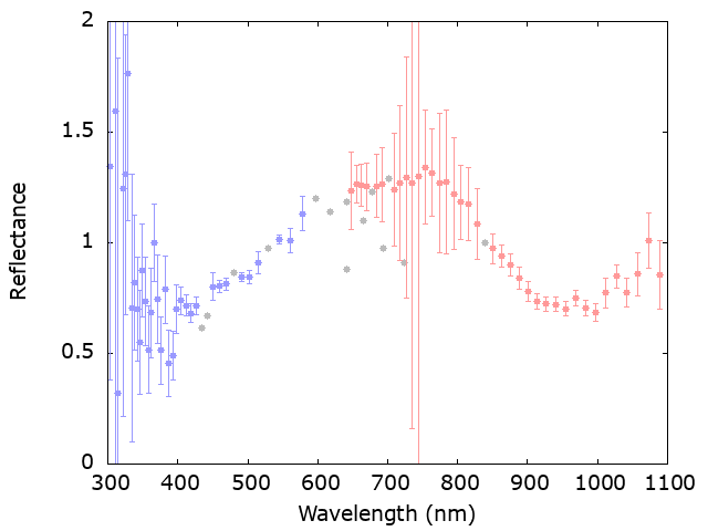
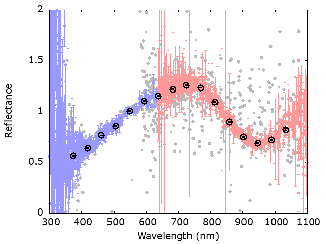
In the vast majority of cases, the BP and RP epoch reflectances superpose in the overlapping range 650 nm 700 nm. However, in some rare cases, the superposition does not occur, as if the RP spectrum has lower flux than the BP one—in some rare cases, a higher flux in RP compared to the BP is observed (Figure 8.14).
Due to these constraints, it has been decided to derive bands from epoch reflectance spectra. The selected wavelengths are the following: 374, 418, 462, 506, 550, 594, 638, 682, 726, 770, 814, 858, 902, 946, 990, and 1034 nm.
The procedure to compute the mean reflectance spectrum is the following:
-
•
consider bands containing all epoch reflectance values measured across the wavelength range nm, nm;
-
•
for each band, the median and the median absolute deviation (m.a.d.) values are computed;
-
•
a -clipping approach is used by filtering all values in each band which are outside the range [median m.a.d., median m.a.d.]; this is done twice in order to remove outlier values;
-
•
a weighted average of each band is computed using the remaining epoch reflectances.
Let the weight of the epoch reflectance at wavelength be the reciprocal square of the uncertainty,
| (8.21) |
The mean reflectance spectrum is computed as the weighted average of the epoch reflectance values,
| (8.22) |
For the computed reflectances, some filtering was applied. A linear regression is computed on the reflectance using the values between 450 and 600 nm. The final reflectance is removed if at least one of the three following tests failed:
-
•
Let be the mean reflectance value between 682 and 770 nm, and be the projected value using the previous linear regression at 726 nm. If , the reflectance is removed from the final output.
-
•
Let be the standard deviation of the reflectances between 682 and 726 nm. If , the reflectance is removed from the final output.
-
•
Let be the interpolated value at 550 nm using the linear regression computed on BP. If , the reflectance is removed from the final output.
Finally, a normalization at nm was introduced for the reflectance. Let be the reflectance value at nm; then
| (8.23) |
sources were removed using these filters. The final number of spectral reflectances computed were using epochs.
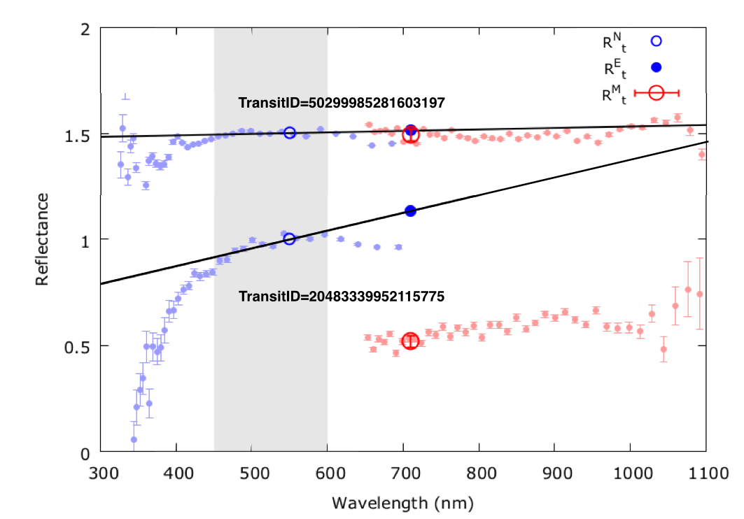
Figure 8.15 exhibits the procedure of computing reflectance.
 |
 |
The information is given in the archive for each asteroid and each wavelength in the table sso_reflectance_spectrum in the field reflectance_spectrum. The wavelength is stored in the same table in the field wavelength. The number of samples (i.e., bands) is stored in the field nb_samples. The number of epoch spectra used to compute the average is stored in the field num_of_spectra.