8.3.2 Signal processing at CCD level

In Gaia DR3, the signal processing at CCD level for SSOs was mainly based on the results of Image Parameter Determination (IPD) performed in IDT and updated by IDU, as described in this document (Section 3.4.2) and in Gaia Collaboration et al. (2016b).

The basic input for IPD consists of ten arrays storing the electron counts collected by the Sky Mapper (SM) and by each of the Astrometric Field CCDs (from AF1 to AF9) during a transit on the focal plane. The whole ensemble of the arrays is represented by a matrix storing the numbers of electrons $C_{s,i,j}$ collected in the $(i,j)$ sample of the $s$th CCD strip, where $s=0$ for SM and $s=1,\mathrm{\dots },9$ for $\mathrm{AF1},\mathrm{\dots },\mathrm{AF9}$, respectively. The ranges of the indices $i=1,\mathrm{\dots },N_{s,x}$ and $j=1,\mathrm{\dots },N_{s,y}$ depend on the particular geometry of the read-out window for the corresponding CCD strip. Index $i$ represents the along-scan position of the sample, whereas $j$ is the across-scan position. The order of the samples corresponds to the read-out sequence so that the sample $(1,1)$ is the first one, $(1,2)$ the second one, and so on. In turn, each sample is the result of the merging (binning) of a sub-array of $B_{s,x}$ pixels in the along-scan direction and $B_{s,y}$ pixels in the across-scan direction, according to the binning rule of each window. Each pixel inside a window is labeled with integers $i^{\prime }=1,\mathrm{\dots },N_{s,x}^{\prime }$ and $j^{\prime }=1,\mathrm{\dots },N_{s,y}^{\prime }$, where $N_{s,x}^{\prime }=B_{s,x}{N}_{s,x}$ and $N_{s,y}^{\prime }=B_{s,y}{N}_{s,y}$ and where $(i^{\prime }=1,j^{\prime }=1)$ is the first read-out pixel. Associated with each $N_{s,x}\times N_{s,y}$ array, a window-related system of coordinate $(x,y)$ is defined in such a way that the centre of the sample $(i,j)$ has coordinates $x=i$ and $y=j$. Another pixel-based coordinate system $(x^{\prime },y^{\prime })$ is defined so that the coordinates of the centre of the pixel $(i^{\prime },j^{\prime })$ are $x^{\prime }=i^{\prime }$ and $y^{\prime }=j^{\prime }$.

The purpose of IPD is to carry out an analysis of the recorded arrays $C_{s,i,j}$ in order to estimate, for each strip, the following parameters of the image:

• •

  the mean position $(x_s,y_s)$ (centroid) of the source during the window integration time, expressed in terms of sample-based coordinates $(x,y)$ or pixel-based coordinates $(x^{\prime },y^{\prime })$;

• •

  the flux $f_s$, namely the number of collected electrons per unit of time, producing the $N_{s,x}\times N_{s,y}$ counts $C_{s,i,j}$.

The IPD algorithm is based on a mathematical signal model $M_{s,i,j}$, depending on the unknown $x_s$, $y_s$, $f_s$ parameters. For details, see Fabricius et al. (2016) and Section 3.3.6 in this document. In a few words, the signal model takes into account the PSF of the instrument together with the level of the local background. Without going into the details discussed in the relevant parts of this documentation, it is worthwile to note that, in the previous data releases DR1 and DR2, IPD relied on a simplified version of the PSF, not necessarily compatible with a source with a SSO-like spectrum. The present release benefits from an improved calibration of the PSF including, in particular, the effect of the source spectral distribution, mitigating the chromaticity bias in centroid determination.

Apart from SM, in the vast majority of cases, the observed windows are one-dimensional, and therefore $N_{s,y}=1$ and the information about the across-scan electron distributions is not recorded. In these cases, it is not possible to determine the $y$ coordinate of the centroid. Moreover, one-dimensional windows do not permit a direct 2D reconstruction of the actual flux, because only the portion of the signal falling within the across-scan limits of the window contribute to the recorded signal, whereas the outside part is lost.

In detail, the list of the data produced by IDT and IDU for each transit and used for SSO signal analysis is the following:

• •

  the value of the magnitude determined on board by the Video Processing Unit (VPU), as a preliminary estimation of the magnitude;

• •

  the window class, a parameter from which it is possible to reconstruct the window geometry for each strip;

• •

  the along-scan and across-scan window coordinates, related to the timing and position of the window in the corresponding CCD;

• •

  the list of along-scan centroids $x_s$;

• •

  the list of the fluxes $f_s$ (photo-electrons per second);

• •

  the list of the across-scan centroids $y_s$, for bi-dimensional windows (SM always included);

• •

  a list of flags describing the quality of the IPD output and the encountered issues.

Unlike along-scan centroids $x_s$, the across-scan coordinates $y_s$ of the centroids are not provided in terms of across-scan coordinates inside the window but rather in terms of across-scan coordinates in the corresponding CCD chip-set.

For the specific purposes of the SSO analysis, the relevant IDT and IDU outputs have been subjected to a general quality control and filtering, described in detail in Section 8.4.1, in order to mitigate the effects of some biases introduced by the peculiarities of the signals of SSOs, not taken into account in IDT and IDU. It is important to stress that, at this stage, the values of the IDT and IDU centroids were not modified in any way, but they were only removed from the data pipeline, whenever they did not fulfil certain quality-control requirements.

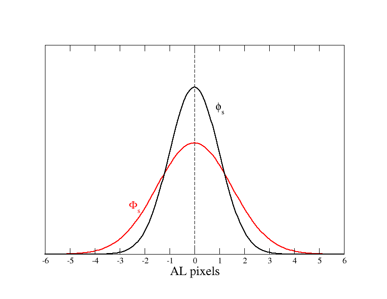
The main difference between the signal of a ‘fixed’ star and the signal of an SSO, both observed by Gaia, consists of an additional AL and AC spread produced by the motion of the moving source and, in several cases, by a non-zero angular size of the image (since some asteroids can be sufficiently large and close not to produce perfectly point-like images). Whereas the effect of a spread due to the angular size of the image is important only in a very minority of cases (about one thousand out of a total of half-a-million SSOs), the angular spread due to the motion of the source plays always an important role and can never be neglected. On the other hand, the IDT and IDU centroids are obtained by fitting the observed signal ${\mathrm{\Phi }}_s$ (in red in Figure 8.8) to the pure PSF ${\varphi }_s$ (in black in Figure 8.8) taking into account all instrumental effects but not including the additional perturbations peculiar to the SSO signals. The best fit is obtained by translating the ${\varphi }_s$ function along scan and rescaling it across scan, in such a way as to maximize an adopted likelihood function (or minimize the ${\chi }^2$ value). Obviously, this process involves the evaluation of the functions ${\mathrm{\Phi }}_s$ and ${\varphi }_s$ at the positions of the window samples. Of course, a rescaling in the ordinates is equivalent to rescaling the integral of ${\varphi }_s$, namely the estimator of the integral of ${\mathrm{\Phi }}_s$, which is the basic information needed to estimate the collected flux together with the centroid position.

Let us assume, for the sake of simplicity, that both ${\mathrm{\Phi }}_s$ and ${\varphi }_s$ are symmetric functions. In this case, if the centroid of the observed ${\mathrm{\Phi }}_s$ is exactly at the centre of the window, the centroid of ${\varphi }_s$ that minimizes the ${\chi }^2$ value is also found in the centre of the window. In other words, it is the real centroid (Figure 8.8, left panel). It does not matter whether the window size is infinite or limited, because the truncation of the signals outside the limits of the window does not modify the symmetry of the configuration.

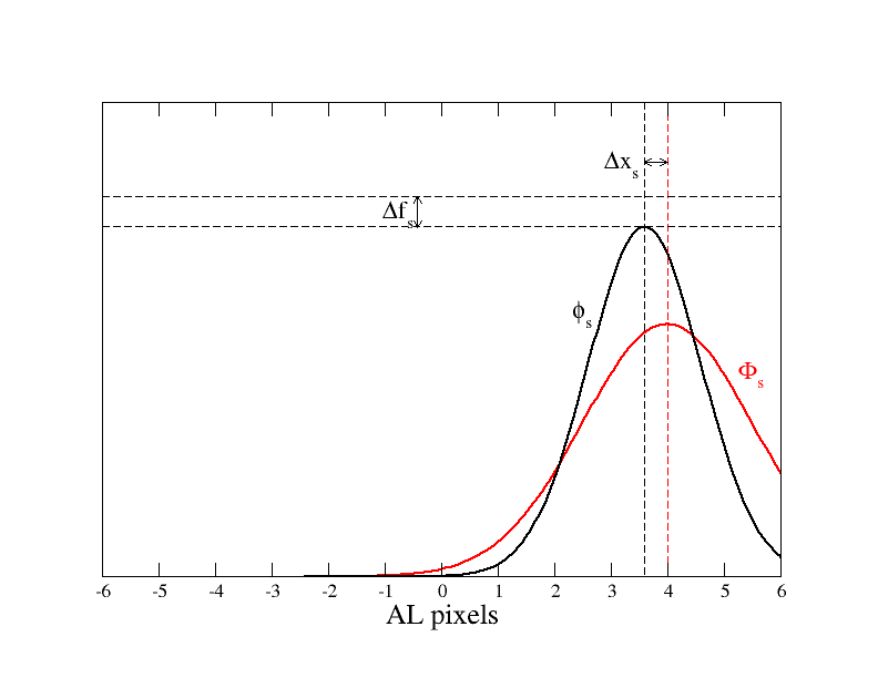The situation is different, however, if the centroid of the observed signal is not exactly at the centre of the window, but close to one of its edges. In this case, the centroid of ${\varphi }_s$ that minimizes the ${\chi }^2$ value is no longer coincident with the centroid of ${\mathrm{\Phi }}_s$. The difference $\mathrm{\Delta }{x}_s$ between the measured centroid and the real centroid is not a purely random error but a systematic bias. The closer the observed signal is to the window edges, the larger is $\mathrm{\Delta }{x}_s$. A similar situation affects the evaluation of the integral of the signal, i.e., the flux of the source, and a systematic off-set $\mathrm{\Delta }{f}_s$ in the flux measurement appears. In more general terms, a non-zero $\mathrm{\Delta }{f}_s$ is present even when the signal is centred in the window, as a consequence of the combination of the different shapes of ${\varphi }_s$ and ${\mathrm{\Phi }}_s$ with their AL truncation. Although, in general, the window width is large enough to make $\mathrm{\Delta }{f}_s$ negligible for centred signals, in most practical situations, the functions ${\varphi }_s$ and ${\mathrm{\Phi }}_s$ are not perfectly symmetric, as assumed so far. As a consequence, a small bias in centroid determination is present even when the signal is close to the window centre. The biases $\mathrm{\Delta }{x}_s$ and $\mathrm{\Delta }{f}_s$ depend on:

• •

  the window geometry and, in particular, the number of AL samples (AL window size);

• •

  the distance of the real centroid from the centre of the window;

• •

  the amount of the spread in the AL direction due to source motion (AL motion of the SSO).

It is important to note that the flux bias $\mathrm{\Delta }{f}_s$, produced by the interplay between the PSF and signal mismatch and the along-scan limited size of the window, has nothing to do with the much more larger flux loss due to the across-scan truncation of the window. As mentioned before, one-dimensional windows do not permit the reconstruction of the total flux of the source. The amount of flux loss has to be determined in other sections of the pipeline of data reduction, specifically devoted to the analysis of photometry (see Section 5.4), together with the calibration of other observational effects. The only one strip that is never affected by an appreciable flux loss is the SM.

For centroiding quality control only, described in Section 8.4.1, a preliminary magnitude estimate $M$ is obtained from the value of the SM flux $f_0$:

where $C$ is the nominal value of the magnitude zero point. Only in cases in which the IDT and IDU IPD for SM provides, for some reason, an invalid result, the value determined on board by VPU is used for $M$.