8.3.3 Astrometric processing
Author(s): Thierry Pauwels, Federica Spoto, Paolo Tanga
Note on magnitudes
Due to the design of the pipeline, at the time of processing, the astrometric reduction does not have the magnitude as derived by CU5 at its disposal. Therefore, it has to use a preliminary magnitude, mostly taken from on-board estimates. It provides a coarse magnitude value, which is accurate enough for the purpose of astrometric reduction which is exclusively used for these purposes. These preliminary magnitudes are not published, since they are overruled by the magnitudes derived by CU5.
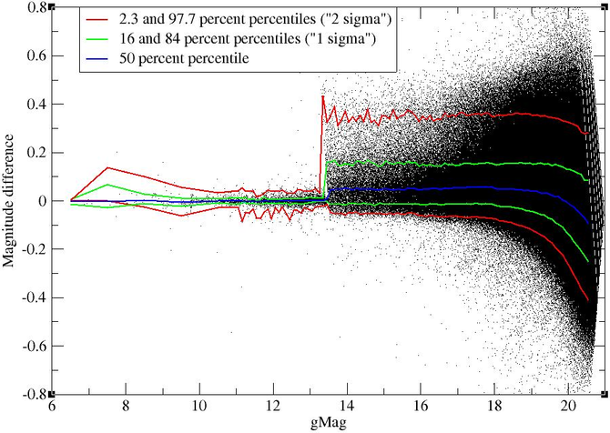
Figure 8.9 shows, for the SSOs, the difference between the preliminary magnitude used by the astrometric reduction module and the final magnitude as given in the catalogue. The horizontal axis shows the mean between both magnitudes. For SSOs brighter than 13.5 mag, differences are typically not larger than 0.01 mag. For fainter objects, we see that the preliminary magnitudes seem to be systematically 0.05 mag fainter than the magnitudes, with typical differences up to 0.2 mag. For very faint objects, however, the preliminary magnitudes seem to be brighter than the magnitudes.
Basic processing
The basic processing of astrometric reduction follows the same procedure as IDT and consists of three consecutive coordinate transformations. For details of these coordinate systems, see Section 4.1, Figure 4.2, Section 4.1.3, Section 4.3.6 and Figure 3.15.
The astrometric reduction is performed for each transit separately. Each transit can contain up to 9 positions: one for each AF CCD strip. Each position is assigned an observation Identifier (ID), which consists of 10 times the transit_id plus the AF strip number, 1 for AF1 up to 9 for AF9. The observation ID is given in the archive in the table sso_observation in the field observation_id.
At input, coordinates are given in the Window Reference System (WRS) and consist of pixel coordinates of the SSO inside the transmitted window along with timings in On-Board Mission Timeline (OBMT), the internal time scale of Gaia (see Section 4.1.6). The origin of the WRS is in the reference pixel of the transmitted window. For the transmitted window, the coordinates in pixels of the window and the binning strategy are given. The timings in OBMT correspond to the time of read-out of the reference pixel of the transmitted window.
The first step of the astrometric data reduction was to compute the epoch of observation, technically the timing of crossing of the fiducial line, i.e., the centre line of the exposure on the CCD. This is half of the exposure time earlier than the reference time, plus a correction for the exact location of the photocentre of the SSO in the transmitted window, and a correction for the size of the transmitted window. The exposure time itself is only dependent on the gating strategy (see Table 1.3) for the window due to the TDI mode of Gaia (see Figure 1.4). The epoch of observation in TDI steps is equal to the AL coordinate of the SSO on the observed strip along the sky, such that position and timing are not independent quantities.
The second step was a conversion from the WRS to the Scanning Reference System (SRS). In the latter system, the coordinates are angles parallel and perpendicular to the scanning direction of Gaia, and the origin of the coordinate system is in the centre of the focal plane of Gaia. This coordinate transformation included the geometric calibration, describing the difference between the nominal and the real positions of the CCDs in the focal plane of Gaia (see Section 4.3.6).
The calibration depended on a series of parameters, all of which were supplied by CU3. To get the correct calibration in the astrometric reduction for SSOs, the arguments supplied by CU3 were passed to the CU3 software. There was, however, one exception, , the effective wave number of the source as used by AGIS. This value was often poorly determined at the time of processing the astrometric reduction of the SSOs. For SSOs, illuminated by the Sun, the solar value of = 0.001561 nm was used for all transits.
The third step was a conversion from the SRS to the Centre-of-Mass Reference System (CoMRS), a non-rotating coordinate system with its origin in the centre of mass of Gaia (see Section 4.1.3).
The last step was a conversion from the CoMRS to the Barycentric Reference System (BCRS), with the origin in the barycentre of the Solar System. This last transformation included the high-precision relativistic correction for aberration, and gave the Right Ascension and Declination of the SSO, i.e., the direction of the unit vector from the centre of mass of Gaia to the SSO (see Section 4.1.3).
In the course of these coordinate transformations, timings were converted from OBMT to Barycentric Coordinate Time (TCB) of the event of observation by Gaia (see Section 4.1.6).
The procedure used the standard coordinate transformations provided by the Gaia software. There was, however, one difference. Since the origin of the light detected, i.e., the SSO, was inside the Solar System, the light path did not extend over the full path through the solar gravity field, so that light bending in the solar gravity field for an SSO is not the same as for a star with the same coordinates.
For the exact amount of light bending, the radial distance from Gaia to the SSO must be known. This last quantity follows from an orbit. Starting in Gaia DR3, no correction was applied for light bending. Communication with potential users of the Gaia data revealed that light bending corrections are best left to the orbit computers. In this respect, the Gaia DR3 data are different from the Gaia DR2 data.
In the same way, no correction was applied for the travel time of the light from the SSO to the spacecraft. The epochs given are the epochs of arrival of the light at the spacecraft.
Positions
Right Ascension and Declination are referred to a system oriented as the International Celestial Reference System (ICRS) and centred on Gaia. The effect of aberration (in its relativistic form) is removed, so that the instantaneous origin of the system is considered to be stationary. This direction is the direction of the unit vector from Gaia to the photocentre of the SSO. The following corrections have not been applied, as they are components of modelling:
-
•
the photocentric shift, giving the difference between the position of the photocentre and the position of the centre of gravity of the SSO, mainly due to the self-shadowing of the SSO;
-
•
the deflection of the light in the solar gravity field;
-
•
the light travel time from the SSO to Gaia.
At each transit, at most 9 positions are given, corresponding to the AF CCDs: AF1 through AF9. The SM CCDs were intended to be processed as well, but the validation showed already at an early stage that positions derived from the SM CCDs have errors much larger than the formal uncertainties resulting from the processing. Therefore, SM positions have systematically been rejected right at the start of the processing.
In many cases, however, there are less than 9 positions in a transit. There can be several reasons for this:
-
1.
Row 4 contains only 8 AF CCDs, rather than 9, so any transit through row 4 can contain no more than 8 positions.
-
2.
There may be various reasons why the software failed to produce a good position for a particular CCD, such as the proximity of a star or a cosmic ray event.
-
3.
A position may have been found to be of too low quality and rejected.
-
4.
The transmitted window is always propagated on board from the SM CCD to the AF CCDs assuming the image to be that of a star. The motion of the SSO in the course of a transit may, however, cause the SSO to leave the transmitted window before the end of the transit. As a result, after the first CCDs, the SSO can exit from the window. Often, in the last CCD in which the SSO is still detected, part of the flux falls already outside the window, causing the photocentre to be shifted towards the centre of the window. In such cases, the last position has also been removed from the output. See Figure 8.10 for an example.
When plotted on a sky map in a Right Ascension–Declination coordinate system, the different positions of a transit of an SSO will not align, and at first sight it may look that the SSO has a zigzag motion in the sky for the duration of a transit (roughly 40 seconds). However, this is an artefact of the observing procedure, and by taking into account the correct error ellipse, one finds that the given positions are perfectly compatible with a linear motion in the sky. The apparent zigzag motion is a consequence of the on-board observing and binning strategy of Gaia. In the SM CCD, the object is detected and a transmitted window is defined, centred on the object. This window is propagated from the SM CCD to all AF CCDs, taking into account the precession of the satellite, but not the motion of the SSO. The precession of the spin axis of Gaia can induce a shift of the transmitted window in the AC direction of up to 4 pixels from one CCD to the next. The exact value, of course, does not correspond to an integer number of pixels, but the windows must be aligned on integer pixels. The shift from one CCD to the next one may thus alternate between different values. Since in the AC direction, in the case of 1D windows, we have no other information on the position than that the SSO is inside the window, the AC component is the centre of the window and the zigzag motion thus reflects only the zigzag motion of the transmitted windows on the different CCDs and not the motion of the SSO.
Figure 8.10 shows most features of the positions and their uncertainties. The figure represents a tiny portion of the sky as observed by Gaia. The horizontal axis is aligned with Right Ascension and the vertical axis with Declination. The scale is in , and the figure represents an area of 400 400 in the sky. The black arrow represents the scanning direction of Gaia, i.e., the black arrow is parallel to the AL axis. The large coloured dots represent the positions as published in the catalogue, while the clouds of little dots represent the uncertainties on the positions. Uncertainties are large perpendicular to the AL direction, and small parallel to the AL direction. The red line connecting the different positions of the transit shows the apparent zigzag motion of the SSO. This apparent zigzag motion is entirely due to the uncertainty on the position perpendicular to the AL direction and the way the transmitted windows are assigned, and is not real. The black line with the coloured squares represents the fit of a linear motion and one can see that a linear motion fits perfectly the positions AF1–AF6. In interpreting this fit, one has to keep in mind that only the AL component of the motion of the objects is real, and that an apparent motion in AC is not real, but an artefact of the observing strategy of Gaia. Careful inspection of the plot shows that AF7 is not in agreement with the derived linear motion, probably because part of the signal fell outside the transmitted window. In AF9, the SSO likely fell completely outside the transmitted window, and the software failed to derive a corresponding position. In this case, the AF7, AF8, and AF9 positions were rejected, and only the AF1–AF6 positions were published.
The positions are given in the archive in the table sso_observation in the fields ra and dec.
Timings
Timings are given in TCB of the event of observation by Gaia, which is the primary timescale for Gaia (see Section 4.1.6 and references therein). Timings correspond to mid-exposure, or more technically, to the instant of crossing of the fiducial line on the CCD by the photocentre of the SSO image. The exact location of the fiducial line depends on the gating strategy applied for that particular window. This gating strategy corresponds to the exposure time. See Section 1.1.3 and Table 1.3 for a detailed explanation of the gating strategy. The timings in TCB are given in the archive in the table sso_observation in the field epoch.
As a convenience for the user, timings have also been converted to Coordinated Universal Time (UTC). UTC is, however, not strictly defined, and for high-precision computations, users should not use UTC timings. The timings in UTC are given in the archive in the table sso_observation in the field epoch_utc.
The uncertainty on the timings is given as 1 TDI cycle, which corresponds roughly to 1 ms. More precise timings would require a detailed modelling of the transfer of charges in the CCDs. However, this is not needed. A typical main-belt asteroid moves at most 10–20 during one TDI cycle which is far less than the uncertainty in the position. Fast moving objects (e.g., NEOs) may move substantially more during one TDI cycle, but the smearing of the image during the 4-s exposure will cause them to have also a larger uncertainty in the position. Therefore, we feel that limiting the precision of the timings to 1 TDI cycle is justified. The uncertainties on the timings (both in TCB and UTC) are given in the archive in the table sso_observation in the field epoch_err.
Observing an SSO by Gaia is considered to be a local Gaia event. Consequently, the timings given are the arrival times at Gaia of the light reflected by the SSO.
Filtering
Filtering is an important activity of astrometric reduction. It ensures that positions that do not really belong to the SSO are rejected, as well as positions that do not meet the high-quality standards. Filtering has been applied both at the level of individual positions (individual CCDs), and at the level of complete transits. Many parameters of the filtering were adjusted by hand, by carefully checking how the software was behaving when treating data of well-known asteroids, and the parameters were optimized to have a minimal number of both false positives and false negatives, i.e., so as to reject a maximum number of bad detections, while minimizing the number of rejected genuine good positions. Needless to say, when treating large numbers of objects in an automatic way, it is inevitable that the data will contain some false positives. In practice, many circumstances are encountered that require an efficient rejection filter. They are listed in what follows.
No data at input
When data was received for astrometric processing from centroiding, positions for which the centroiding module failed to fit a PSF or Line Spread Function (LSF) to the image, were already missing. These positions have obviously been filtered out.
Weird cases
Some weird cases were too difficult to treat or could give rise to positions of which the accuracy could not be guaranteed. These positions have been rejected right at the start of the processing. They include:
-
•
all positions from the SM CCDs;
-
•
any position suspected to be contaminated by a nearby star (*);
-
•
any position that had all samples equal to zero (*);
-
•
any position that had eliminated samples;
- •
-
•
any position that was affected by a non-nominal gating;
-
•
any position that was too close to the celestial pole (*);
-
•
any position with an invalid value for distToLastCi (the distance in TDIs from the last charge injection, see Section 3.3.3);
-
•
any position for which no attitude is available for the corresponding epoch;
-
•
any position with an epoch for which no Gaia ephemeris is available (*);
-
•
any position for which the attitude is of known too poor quality;
-
•
any position for which acRateParams is not between 1.2 and 1.2 (see Section 4.3.5);
-
•
all positions of any transit for which the preliminary magnitude is fainter than 22.
Filters marked with an asterisk were implemented in the software, but it turned out that not a single position was rejected by these filters.
Some of the filters depend on the magnitude of the SSO. At the time of processing of the SSO, the astrometric reduction did not have the high-precision photometry of the photometric pipeline at its disposal. Therefore it could only rely on the preliminary magnitude. These are not published, but should not deviate too much from the published magnitudes.
As already mentioned above, previous runs have shown that errors of SM positions are much larger than the computed uncertainties, and are of insufficient quality. Other filters could have rejected these positions, because they would not be in agreement with the derived linear motion of the SSO, but some of these SM data could just be by chance in agreement and not be rejected, or they could influence the fitted linear motion causing other genuine positions to be rejected. To avoid this to happen, they were rejected a priori.
In Gaia DR2, positions from truncated windows were rejected. However, truncated windows turned out to be less of a problem than initially thought. Therefore, starting with Gaia DR3, truncated windows have no longer been rejected, leaving the positions of lesser quality, if any, to be rejected by the other filters.
Positions too close to the celestial pole suffer from all sorts of ill-defined conditions. An example would be the case where the error ellipse would include the celestial pole. Although from a theoretical point of view it is not difficult to treat these cases, this would cause a lot of practical problems. For Gaia DR3, the minimal distance to the celestial pole has been set to 1, but in fact not a single such case was present in the Gaia DR3 data.
All other cases were reported by upstream processes, and interested users should refer to the appropriate sections, as mentioned above, for more details.
Uncertainty-magnitude relation
When analysing the relation between the AL uncertainties coming from the centroiding process and the magnitude for confirmed real detections of SSOs, they all lie between rather tight limits. Positions with reported uncertainties unrealistically large or small for the given magnitude are clearly not detections of SSOs. This can be used to define a first, simple selection criterion. After careful investigation, and several fine-tunings, we defined the following conditions for Gaia DR3:
| (8.5) |
where is the AL component of the computed uncertainty from the centroiding, including the added excess noise (see Subsection 8.3.4), and where and are the corresponding minimum and maximum allowed values,
| (8.6) |
| (8.7) |
where is the preliminary magnitude. Furthermore,
| (8.8) |
is the contribution to correct for the effect of excess noise (see Subsection 8.3.4), and
| (8.9) |
the contribution taking into account the centroiding uncertainty. All positions not satisfying Equation 8.5 were rejected.
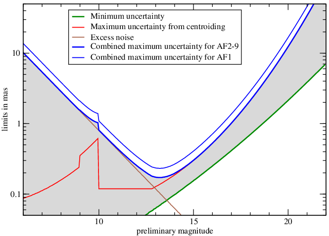
Figure 8.11 shows the relation defined by Equation 8.5. In green is the minimal uncertainty as a function of magnitude. In blue is the maximum allowed uncertainty as a function of magnitude: the thick blue line is for AF2–9 and the thinner blue line for AF1. The two contributions to the maximum uncertainty are shown in red and brown. As can be seen, for bright objects, the excess noise is dominating, implying that the filter will no longer be effective. The grey-shaded region is the range of allowed uncertainties for AF2–9. AF1 has been found empirically to have systematically slightly larger uncertainties. Therefore, uncertainties for AF1 were allowed to be 1.35 times larger than for AF2–9.
Ideally, the check should not have included the excess noise, and should have been done purely on the centroiding uncertainty. However, the inclusion of the excess noise to the error budget happened too close to the deadline of Gaia DR3, and we had to opt for a quick solution.
Fitting a linear motion
An SSO will show a linear motion on the sky in the course of a single transit. Even for extremely fast and close-by objects, after using a gnomonic projection on a plane tangential to the sky, the motion will be linear, implying that both space coordinates are linear functions of time. An efficient way to remove false detections is to check the linearity of the motion and whether all positions are in agreement with the regression line within the computed uncertainties. This way, we can efficiently reject detections for which part of the flux falls outside the transmitted window, causing the position to be shifted to the window centre.
The adopted procedure was as follows. First, a linear regression of the positions as a function of epoch was computed, taking into account the proper weights resulting from the uncertainties. In this process, the SM position had already been removed. Whenever the complete set of positions was found to be consistent, i.e., whenever all residuals of the fit were smaller than a given threshold, the transit with all its positions was accepted. If at least one residual was found to be too large, then an iterative process was started, where, in the first iteration, one position was removed from the transit and, in each iteration, one more position was removed until a minimum set was reached. The minimum number of positions in a transit to check for consistency is user selectable but cannot be lower than 3, since any set of only two positions will be consistent with a linear motion.
In the th iteration, the software tried all possible combinations of the transit with positions removed. If it found one single combination to be a consistent set, the transit was accepted, but the positions that had to be removed to get the consistent set were considered as outliers, and were rejected. If, for all the sets, none was found to be consistent, i.e., there was still at least one residual which was too large, this meant that no linear motion could be found with positions removed, or that at least positions were bad. A next iteration was then started with positions removed. If, however, more than one set of positions was found in the th iteration, to be consistent, the software could not decide which positions were the outliers to be rejected. The threshold was then relaxed, and the whole procedure was repeated starting with all positions and gradually removing more and more positions from the transit, until either a single set was found to be consistent (but now using the relaxed threshold), in which case the transit was accepted with the positions rejected to get the consistent set; or until more than one consistent set was found with the same number of positions removed, in which case the threshold was again relaxed, until a maximum value of the threshold was reached.
If the maximum value of the threshold was reached, and there was still more than one consistent set with the same number of positions, the transit was considered to be of low quality, and was rejected as a whole. If the transit at the start contained less than the minimal number of positions to search for consistent sets (e.g., because the SSO was so fast that it left the transmitted window after two CCDs and that this caused already all other positions to be rejected on the basis of the uncertainty-magnitude relation), the complete transit was accepted, without any position being rejected. This means that the consistency check was in fact by-passed. If, however, the procedure reached the minimal number of positions to search for consistent sets without finding any, the transit was considered not to belong to an SSO, and the complete transit was rejected.
For Gaia DR3, the following parameters have been set:
-
•
the threshold for the residual was set to 2 sigma, here meaning that residuals considered as 2D vectors, should not extend further than twice the error ellipse;
-
•
the maximum relaxed threshold for the residual was set to 4 sigma;
-
•
the increment to relax the threshold was set to 0.1 sigma;
-
•
the minimum number of positions in a consistent set was set to 3, i.e., at least 4 positions were required to be able to identify an outlier.
Minimum number of positions in a transit
After applying all the other filters, a final check was to assess how many positions were left in a transit. Since the search for consistent positions cannot be performed with less than three positions, it is risky to accept transits with less than three positions. The minimum number of positions left in a transit is user selectable and any transit left with less than this number of positions is rejected as a whole. For Gaia DR3, however, with an a priori list of transits to be processed that were already identified as belonging to SSOs and with a further quality check downstream by fitting an orbit to the positions, it was found safe to set this limit to 2. Extensive checks have shown that the vast majority of the transits with only two positions are good positions that belong to real SSOs. This means that only transits with a single position left have been rejected.
Magnitude limit
Unlike in Gaia DR2, in Gaia DR3, there was no lower limit on the magnitude. This could be achieved thanks to the inclusion of the excess noise in the error budget (see Subsection 8.3.4).
In the archive
The results of the filtering are given in the archive in the table sso_observation in the fields astrometric_outcome_ccd and astrometric_outcome_transit. astrometric_outcome_ccd will give for each rejected CCD in the transit why it was rejected. astrometric_outcome_transit will only be given for non-rejected transits, and will otherwise only signal transits that may be of lower quality.
Additional items in the archive
The astrometric reduction generates also a few additional output items that are necessary or useful for orbit computers. The barycentric position of the satellite Gaia in the Solar System at the epoch of each position is given in the archive in the table sso_observation in the fields x_gaia, y_gaia, and z_gaia, whereas the barycentric velocity of Gaia in the Solar System is given in the archive in the table sso_observation in the fields vx_gaia, vy_gaia, and vz_gaia. In a similar way, the geocentric position and velocity of Gaia are given in the archive in the table sso_observation in the fields x_gaia_geocentric, y_gaia_geocentric, z_gaia_geocentric, vx_gaia_geocentric, vy_gaia_geocentric, and vz_gaia_geocentric. Finally, the archive gives also the position angle of the scan, i.e., the angle between the North-South direction on the sky and the scanning direction of the satellite (the orientation of the focal plane) in the sky. This is given in the archive in the table sso_observation in the field position_angle_scan.