8.4.2 Quality control of Astrometry
Author(s): Thierry Pauwels
Filtering at transit level
The different filters used in the astrometric reduction and that filter out complete transits, with a code for further referencing, are listed in Table 8.7. Filters that did not reject a single transit are omitted from this list.
| code | filter |
| T-04 | Transit rejected because of acRateParams out of range. |
| T-11 | Transit rejected because no linear motion can be fit. |
| T-12 | Transit rejected because of ambiguous outlier rejection. |
| T-13 | Transit rejected because not enough positions left after all filters on individual positions were applied. In Gaia DR3, this means that less than 2 positions were left in the transit. |
All these filters will remove complete transits with all their positions. They are listed in the sequence in which they are encountered in the pipeline. Transits thus filtered out leave no trace in the catalogue.
Table 8.8 lists, per filter and per magnitude bin, how many transits were filtered out in the astrometric reduction. A magnitude bin is to be understood as the range from to . The first line lists the number of transits at input for each magnitude bin; the last line lists the number of transits at output. The last column gives the total for all magnitude bins.
| gMag | 6 | 7 | 8 | 9 | 10 | 11 | 12 | 13 | 14 | 15 | 16 | 17 |
| At input | 35 | 29 | 54 | 157 | 537 | 1062 | 2667 | 5144 | 10042 | 18328 | 45642 | 143918 |
| T-04 | 0 | 0 | 0 | 0 | 0 | 0 | 0 | 0 | 1 | 1 | 0 | 0 |
| T-11 | 2 | 0 | 2 | 1 | 0 | 2 | 9 | 1 | 8 | 15 | 85 | 255 |
| T-12 | 0 | 0 | 0 | 2 | 0 | 0 | 6 | 0 | 0 | 2 | 8 | 21 |
| T-13 | 4 | 6 | 10 | 4 | 19 | 46 | 141 | 336 | 715 | 1347 | 4476 | 13212 |
| At output | 29 | 23 | 42 | 150 | 518 | 1014 | 2511 | 4807 | 9318 | 16963 | 41073 | 130430 |
| gMag | 18 | 19 | 20 | total |
| At input | 492153 | 1415023 | 1361276 | 3496067 |
| T-04 | 6 | 8 | 7 | 23 |
| T-11 | 666 | 1684 | 4300 | 7030 |
| T-12 | 69 | 268 | 821 | 1197 |
| T-13 | 47174 | 108794 | 93123 | 269407 |
| At output | 444238 | 1304269 | 1263025 | 3218410 |
Table 8.9 lists, per filter and per magnitude bin, which percentage of the remaining (after all previous filters were applied) transits were filtered out in the astrometric reduction. The last line combines the numbers for all filters together. The last column gives the total for all magnitude bins.
| gMag | 6 | 7 | 8 | 9 | 10 | 11 | 12 | 13 | 14 | 15 | 16 | 17 | 18 | 19 | 20 | total |
| T-04 | 0.0 | 0.0 | 0.0 | 0.0 | 0.0 | 0.0 | 0.0 | 0.0 | 0.0 | 0.0 | 0.0 | 0.0 | 0.0 | 0.0 | 0.0 | 0.0 |
| T-11 | 5.7 | 0.0 | 3.7 | 0.6 | 0.0 | 0.2 | 0.3 | 0.0 | 0.1 | 0.1 | 0.2 | 0.2 | 0.1 | 0.1 | 0.3 | 0.2 |
| T-12 | 0.0 | 0.0 | 0.0 | 1.3 | 0.0 | 0.0 | 0.2 | 0.0 | 0.0 | 0.0 | 0.0 | 0.0 | 0.0 | 0.0 | 0.1 | 0.0 |
| T-13 | 12.1 | 20.7 | 19.2 | 2.6 | 3.5 | 4.3 | 5.3 | 6.5 | 7.1 | 7.4 | 9.8 | 9.2 | 9.6 | 7.7 | 6.9 | 7.7 |
| Total | 17.1 | 20.7 | 22.2 | 4.5 | 3.5 | 4.5 | 5.8 | 6.6 | 7.2 | 7.4 | 10.0 | 9.4 | 9.7 | 7.8 | 7.2 | 7.9 |
We see that filters at transit level reject only a small number of transits, if we take into account that filter T-13 is in fact the result of filtering at CCD level, see Subsection 8.4.2. At input, 3 496 067 transits were received for the astrometric reduction and, at output, there were 3 218 410 transit left, which means a rejection rate of 7.9 %.
Filtering at CCD level
The different filters used in the astrometric reduction and that filter out individual positions, with a code for further referencing, are listed in Table 8.10. Again, filters that did not reject a single position are omitted from this list. Note that filters that act on complete transits, in fact also filter out all the positions from those transits. Therefore, in the tables with the effect of filtering at CCD level, also the filters acting on complete transits are listed.
| code | filter |
| C-03 | Position rejected because no centroid could be derived. |
| C-05 | Position rejected because of distToLastCi outside valid range. |
| C-06 | Position rejected because of eliminated samples, AOCS update, or non-nominal gating. |
| C-07 | Position rejected because there is no attitude available for that epoch. |
| C-08 | Position rejected because it does not satisfy the uncertainty-magnitude relation. |
| C-09 | Position rejected because the epoch corresponds to known bad attitude. |
| C-10 | Position rejected because it does not agree with the derived linear motion. |
These filters are listed in the sequence in which they are encountered in the pipeline, with a common numbering for transit-based filters and CCD-based filters. Individual positions thus filtered out are no longer present in the catalogue. However, if the corresponding transit is still present, astrometric_outcome_ccd gives a code for all CCDs of the transit, also those that have been rejected, so that the user can check why a particular position has been rejected.
| gMag | 6 | 7 | 8 | 9 | 10 | 11 | 12 | 13 | 14 | 15 | 16 |
| At input | 311 | 256 | 480 | 1403 | 4736 | 9432 | 23642 | 45503 | 88952 | 162288 | 404160 |
| C-03 | 77 | 56 | 50 | 195 | 549 | 1279 | 3052 | 4324 | 7777 | 14192 | 86480 |
| T-04 | 0 | 0 | 0 | 0 | 0 | 0 | 0 | 0 | 9 | 8 | 0 |
| C-05 | 0 | 1 | 1 | 2 | 14 | 13 | 3 | 0 | 1 | 0 | 6 |
| C-06 | 0 | 3 | 0 | 0 | 19 | 29 | 145 | 229 | 462 | 731 | 949 |
| C-07 | 0 | 0 | 0 | 0 | 0 | 0 | 2 | 0 | 20 | 10 | 68 |
| C-08 | 0 | 0 | 0 | 2 | 0 | 9 | 35 | 91 | 555 | 1720 | 5701 |
| C-09 | 32 | 41 | 87 | 25 | 105 | 253 | 803 | 1960 | 4495 | 8412 | 19771 |
| C-10 | 28 | 19 | 41 | 140 | 196 | 478 | 1234 | 632 | 848 | 1082 | 1793 |
| T-11 | 8 | 0 | 7 | 7 | 0 | 8 | 34 | 3 | 24 | 45 | 271 |
| T-12 | 0 | 0 | 0 | 14 | 0 | 0 | 40 | 0 | 0 | 13 | 49 |
| T-13 | 0 | 0 | 0 | 1 | 2 | 4 | 7 | 18 | 38 | 69 | 1009 |
| At output | 166 | 136 | 294 | 1017 | 3851 | 7359 | 18287 | 38246 | 74723 | 136006 | 288063 |
| gMag | 17 | 18 | 19 | 20 | total |
| At input | 1274641 | 4357768 | 12529392 | 12055043 | 30958007 |
| C-03 | 241955 | 777163 | 2029657 | 2002493 | 5169299 |
| T-04 | 0 | 44 | 46 | 53 | 160 |
| C-05 | 14 | 41 | 116 | 117 | 329 |
| C-06 | 3333 | 14046 | 51129 | 56954 | 128029 |
| C-07 | 100 | 495 | 1320 | 1823 | 3838 |
| C-08 | 21092 | 82251 | 347216 | 499040 | 957712 |
| C-09 | 65485 | 194538 | 439493 | 377882 | 1113382 |
| C-10 | 5312 | 16261 | 41777 | 49920 | 119761 |
| T-11 | 781 | 2028 | 5165 | 13280 | 21661 |
| T-12 | 126 | 387 | 1542 | 3866 | 6037 |
| T-13 | 2470 | 12630 | 29389 | 23546 | 69183 |
| At output | 933973 | 3257884 | 9582542 | 9026069 | 23368616 |
Table 8.11 lists, per filter and per magnitude bin, how many positions were filtered out in the astrometric reduction. Again, a magnitude bin is to be understood as the range from to . The first line lists the number of positions at input for each magnitude bin, the last line the number of positions at output. The last column gives the total for all magnitude bins. Transit-based filters are also mentioned, since they effectively remove all the remaining positions of the transit. Filters are listed in the sequence they are encountered in the software. Note that SM positions had already been discarded right from the start and are not taken into consideration in these numbers.
| gMag | 6 | 7 | 8 | 9 | 10 | 11 | 12 | 13 | 14 | 15 | 16 |
| C-03 | 24.8 | 21.9 | 10.4 | 13.9 | 11.6 | 13.6 | 12.9 | 9.5 | 8.7 | 8.7 | 21.4 |
| T-04 | 0.0 | 0.0 | 0.0 | 0.0 | 0.0 | 0.0 | 0.0 | 0.0 | 0.0 | 0.0 | 0.0 |
| C-05 | 0.0 | 0.5 | 0.2 | 0.2 | 0.3 | 0.2 | 0.0 | 0.0 | 0.0 | 0.0 | 0.0 |
| C-06 | 0.0 | 1.5 | 0.0 | 0.0 | 0.5 | 0.4 | 0.7 | 0.6 | 0.6 | 0.5 | 0.3 |
| C-07 | 0.0 | 0.0 | 0.0 | 0.0 | 0.0 | 0.0 | 0.0 | 0.0 | 0.0 | 0.0 | 0.0 |
| C-08 | 0.0 | 0.0 | 0.0 | 0.2 | 0.0 | 0.1 | 0.2 | 0.2 | 0.7 | 1.2 | 1.8 |
| C-09 | 13.7 | 20.9 | 20.3 | 2.1 | 2.5 | 3.1 | 3.9 | 4.8 | 5.6 | 5.8 | 6.4 |
| C-10 | 13.9 | 12.3 | 12.0 | 11.9 | 4.8 | 6.1 | 6.3 | 1.6 | 1.1 | 0.8 | 0.6 |
| T-11 | 4.6 | 0.0 | 2.3 | 0.7 | 0.0 | 0.1 | 0.2 | 0.0 | 0.0 | 0.0 | 0.1 |
| T-12 | 0.0 | 0.0 | 0.0 | 1.4 | 0.0 | 0.0 | 0.2 | 0.0 | 0.0 | 0.0 | 0.0 |
| T-13 | 0.0 | 0.0 | 0.0 | 0.1 | 0.1 | 0.1 | 0.0 | 0.0 | 0.1 | 0.1 | 0.3 |
| Total | 46.6 | 46.9 | 38.8 | 27.5 | 18.7 | 22.0 | 22.7 | 15.9 | 16.0 | 16.2 | 28.7 |
| gMag | 17 | 18 | 19 | 20 | total |
| C-03 | 19.0 | 17.8 | 16.2 | 16.6 | 16.7 |
| T-04 | 0.0 | 0.0 | 0.0 | 0.0 | 0.0 |
| C-05 | 0.0 | 0.0 | 0.0 | 0.0 | 0.0 |
| C-06 | 0.3 | 0.4 | 0.5 | 0.6 | 0.5 |
| C-07 | 0.0 | 0.0 | 0.0 | 0.0 | 0.0 |
| C-08 | 2.0 | 2.3 | 3.3 | 5.0 | 3.7 |
| C-09 | 6.5 | 5.6 | 4.4 | 4.0 | 4.5 |
| C-10 | 0.6 | 0.5 | 0.4 | 0.5 | 0.5 |
| T-11 | 0.1 | 0.1 | 0.1 | 0.1 | 0.1 |
| T-12 | 0.0 | 0.0 | 0.0 | 0.0 | 0.0 |
| T-13 | 0.3 | 0.4 | 0.3 | 0.3 | 0.3 |
| Total | 26.7 | 25.2 | 23.5 | 25.1 | 24.5 |
Table 8.12 lists, per filter and per magnitude bin, which percentage of the remaining (after all previous filters were applied) positions were filtered out in the astrometric reduction. The last line combines the numbers for all filters together. The last column gives the total for all magnitude bins.
We see that most filters tend to reject more brighter objects than fainter objects. The big exception is filter C-08, which filters more faint objects. We also see that filter T-13, which seemed to filter out a lot of transits, in fact, removes only few positions. This is because transits removed by filter T-13 had only 0 or 1 position left. At input, the astrometric reduction module received 30 958 007 positions in the focal plane, including those without derived centroid. This comprises 9 AF positions for rows 1–3 and 5–7, and 8 AF positions for row 4. At output, the astrometric reduction module produced 23 368 616 positions in the sky, which corresponds to a rejection rate of 24.5 %. Rejected positions are mainly those for which the SSO had left the transmitted window or where the object was too close to the window border to produce a reliable position.
Comparison of residuals and uncertainties
Systematic-type and random-type residuals
In this section, the residuals (observed positions minus computed positions) as derived by orbital fitting are checked against their expected distribution, as derived from the computed random and systematic uncertainties on the positions. In the case of 1D windows, we can compare only the AL components.
In the same way as for the uncertainties, we can define systematic-type and random-type residuals. The former is defined as the average residual over the complete transit and termed the SYST residual. The latter is defined as the difference between the total residual and the SYST residual of the transit and termed the RAND residual.
With these definitions, the dispersion of the RAND residuals is expected to be
| (8.28) |
and the dispersion of the SYST residuals is expected to be
| (8.29) |
where refers to a residual, is the uncertainty of the position, is the dispersion of the quantity between braces, and the summation is over all positions of the transits remaining after all filtering has been applied.
If we then divide each residual by its expected dispersion, and plot these, in the ideal case, we should get a standard normal distribution. The real plots show us how close we are to the ideal case.
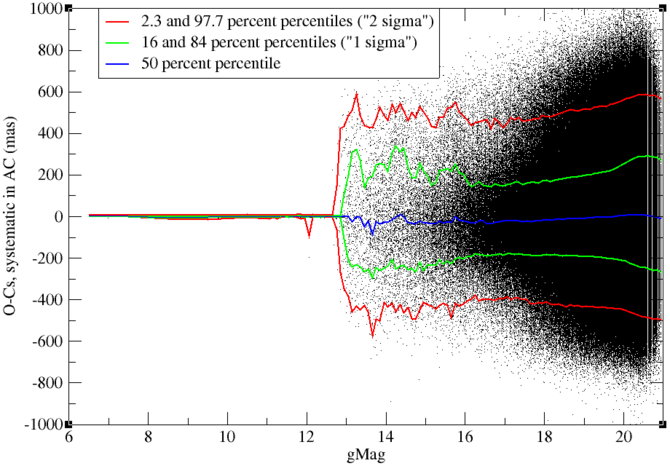
In the following subsections, we give plots for different residuals as a function of preliminary magnitude. In each plot, the black dots represent the data points. Note that, for RAND residuals, there are as many data points as there are positions, whereas, for SYST residuals, there are as many data points as there are transits. The curves represent percentiles. These are computed in magnitude bins of 0.1 mag, if there are enough data points. If that is not the case, magnitude bins have been made larger. The blue lines are the median lines, i.e., the 50-% percentile. In the ideal case, it should be the mean of the Gaussian distribution. The green curves are the 16-% and 84-% percentiles, corresponding, in the ideal case, to the 1-sigma values of a Gaussian distribution. The blue curves are the 2.3-% and 97.7-% percentiles, corresponding, in the ideal case, to the 2-sigma values of a Gaussian distribution.

Random-type residual in AL
Figure 8.17 shows the AL component of the RAND residuals of the individual positions. As expected, the residuals become larger when the object becomes fainter. Less expected is that the residuals become minimal around magnitude 14, and increase again for brighter objects. The cause is not understood, but it was the motivation to add the empirical excess noise to the error budget, see Subsection 8.3.4.
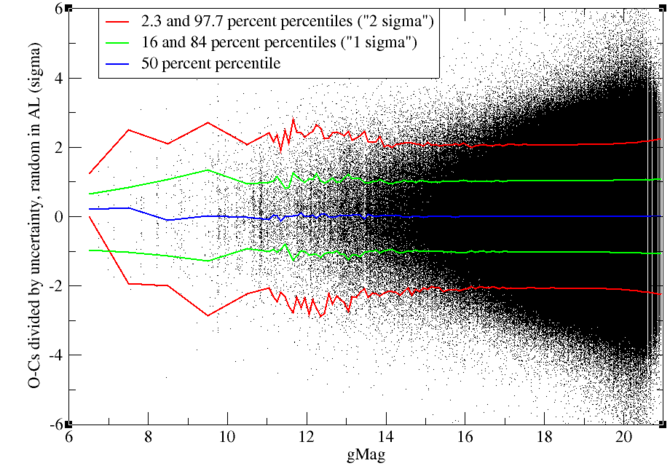
Figure 8.18 shows the same residuals as Figure 8.17, but divided by their expected dispersion as computed by Equation 8.28. The blue, green, and red curves, representing the percentiles, are close to their expected positions, respectively 0, 1, and 2, showing that the RAND residuals in AL really behave as expected, thanks to the addition of the excess noise.
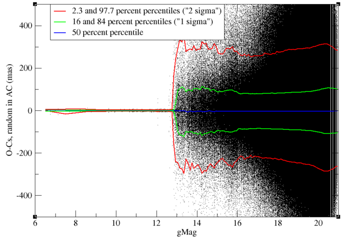
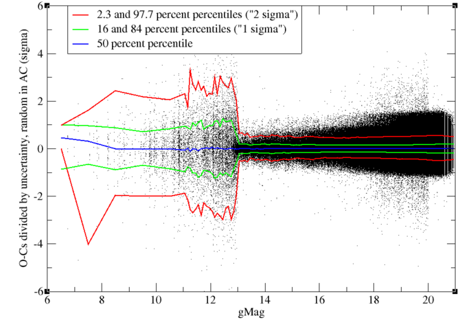
Random-type residual in AC
Figure 8.19 shows the AC component of the RAND residuals of the individual positions. In this case, for SSOs fainter than magnitude 13, the vast majority have 1D windows, so that the residuals are comparable to the window size. SSOs brighter than magnitude 13 have 2D windows and have much smaller residuals. When divided by the expected dispersion of the residual, see Figure 8.20, residuals of objects brighter than magnitude 13 behave as expected, in the same way as the AL residuals. Objects fainter than magnitude 13 have smaller residuals than “expected”, but this is due to an oversimplification of the computation of the uncertainty in the positions, as explained in Subsection 8.3.4.
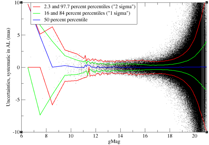
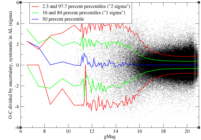
Systematic-type residual in AL
Figure 8.21 shows the AL component of the SYST residuals of the individual positions. At first sight, the behaviour is similar to the behaviour of the RAND residuals. But when divided by the expected dispersion of these residuals, as shown in Figure 8.22, we see a rather different picture. Residuals are smaller than expected by a factor of 2–3 for SSOs fainter than magnitude 18 but about twice as large as expected for SSOs brighter than magnitude 14.
The cause of this behaviour is not understood. One could think of an underestimate of the SYST uncertainty of the attitude and, at first sight, a constant residual of 0.5 between magnitudes 12 and 15 seems to confirm this. But this could never explain the minimum in the residuals around magnitude 17, where they are around 0.3 , since the uncertainty on the attitude is a constant independent of the magnitude, to be added to the error budget.
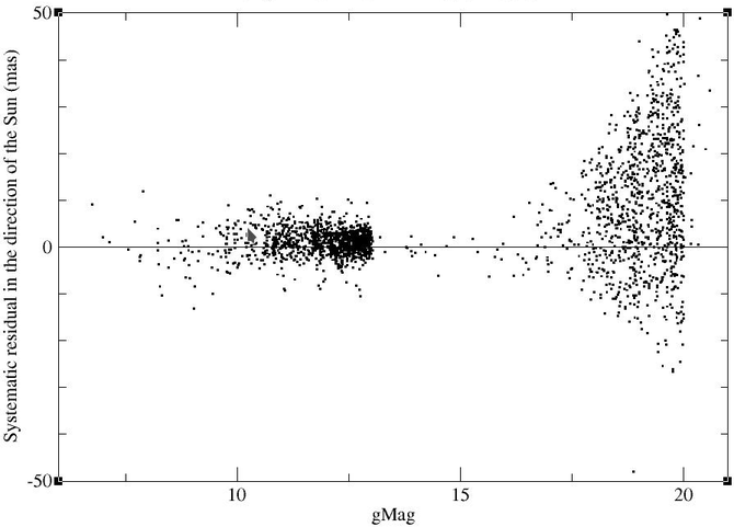
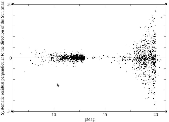
Another possible cause that we investigated is the photocentric shift. Figure 8.23 shows the component of the residual pointing in the sky towards the Sun. Figure 8.24 shows the component of the residual being perpendicular to the direction of the Sun in the sky. Both plots are obviously restricted to the SSOs with 2D windows. At first sight, the asymmetry in the residuals towards the Sun and the lack of asymmetry in the residuals perpendicular to this direction seems to confirm that the photocentric shift may be the cause. However, a measurable photocentric shift should be restricted to bright objects, and should increase with decreasing magnitude. A photocentric shift of nearly 5 is impossible for a 20th-magnitude SSO.
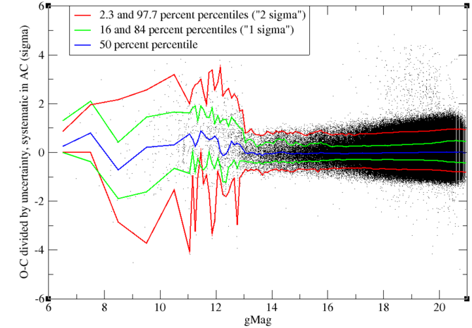
Systematic-type residual in AC
2D windows
In the case of 2D windows, we have also the full positional information in the AC direction. All objects brighter than magnitude 13 will, in principle, have 2D windows (note that this concerns only a small proportion of all transits), but also a limited number of faint objects will have 2D windows. One can also wonder whether, for faint objects, the behaviour in AL is the same for those with 1D or 2D windows.
| mag | Number of positions |
| 7 | 256 |
| 8 | 480 |
| 9 | 1403 |
| 10 | 4736 |
| 11 | 9432 |
| 12 | 21078 |
| 13 | 406 |
| 14 | 160 |
| 15 | 159 |
| 16 | 283 |
| 17 | 797 |
| 18 | 3509 |
| 19 | 5365 |
| 20 | 347 |
| total | 48722 |
Table 8.13 gives, for each magnitude bin, the number of 2D positions at input of the astrometric reduction. Note the small numbers in the magnitude range 13–18, so that statistics in this magnitude range will not tell us a lot.
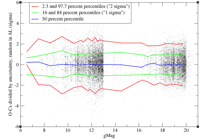
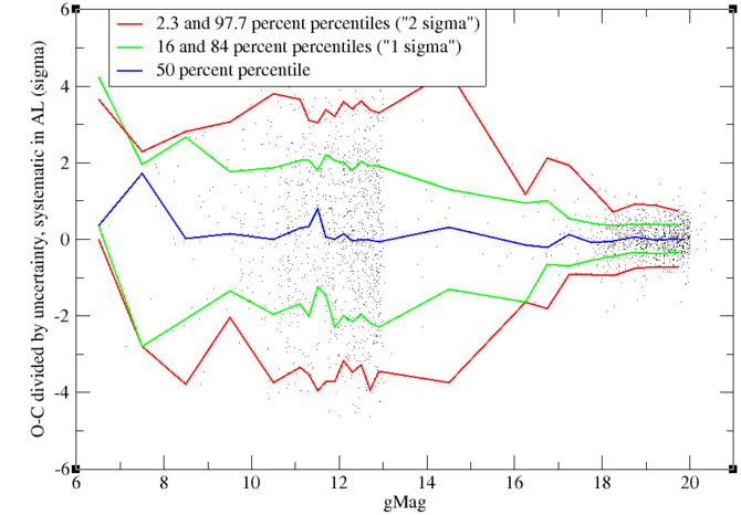
Figure 8.27 and Figure 8.28 give the random-type and systematic-type residuals divided by their computed dispersion, restricted to 2D windows. Comparison with Figure 8.18 and Figure 8.22 gives immediately that AL residuals behave the same for 1D and 2D windows.
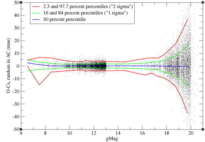
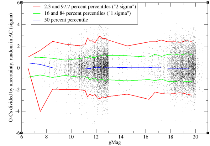
Figure 8.29 and Figure 8.30 give the RAND residuals in AC for 2D windows and the same residuals divided by their computed uncertainty. We see a behaviour very similar to the RAND residuals in AL. However, looking at the scale we see immediately that residuals in AC are a lot larger than residuals in AL for comparable magnitude. This has of course to do with the larger pixel size in AC.
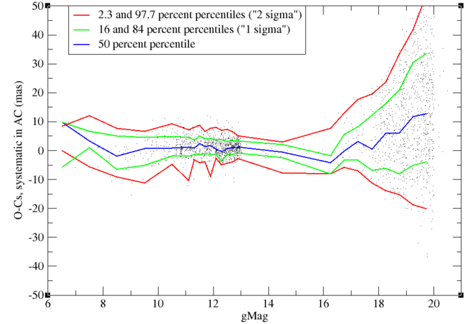
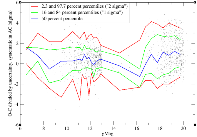
Figure 8.31 and Figure 8.32 give the SYST residuals in AC for 2D windows and the same residuals divided by their computed uncertainty. Here we notice some unexplained features: for faint objects, the residuals are substantially larger than expected (this is the reverse of AL), whereas we see also an asymmetry in the residuals, which is more pronounced for faint objects than for bright objects.
| gMag | 6 | 7 | 8 | 9 | 10 | 11 | 12 | 13 | 14 | 15 | 16 |
| C-03 | 24.8 | 21.9 | 10.4 | 13.9 | 11.6 | 13.6 | 13.3 | 21.4 | 20.0 | 34.0 | 20.8 |
| T-04 | 0.0 | 0.0 | 0.0 | 0.0 | 0.0 | 0.0 | 0.0 | 0.0 | 0.0 | 0.0 | 0.0 |
| C-05 | 0.0 | 0.5 | 0.2 | 0.2 | 0.3 | 0.2 | 0.0 | 0.0 | 0.0 | 0.0 | 0.0 |
| C-06 | 0.0 | 1.5 | 0.0 | 0.0 | 0.5 | 0.4 | 0.8 | 5.0 | 2.3 | 0.0 | 0.0 |
| C-07 | 0.0 | 0.0 | 0.0 | 0.0 | 0.0 | 0.0 | 0.0 | 0.0 | 0.0 | 0.0 | 0.0 |
| C-08 | 0.0 | 0.0 | 0.0 | 0.2 | 0.0 | 0.1 | 0.1 | 0.0 | 3.2 | 21.0 | 5.4 |
| C-09 | 13.7 | 20.9 | 20.3 | 2.1 | 2.5 | 3.1 | 3.7 | 2.6 | 7.4 | 0.0 | 3.3 |
| C-10 | 13.9 | 12.3 | 12.0 | 11.9 | 4.8 | 6.1 | 6.2 | 4.7 | 6.2 | 2.4 | 2.9 |
| T-11 | 4.6 | 0.0 | 2.3 | 0.7 | 0.0 | 0.1 | 0.2 | 0.0 | 0.0 | 0.0 | 0.0 |
| T-12 | 0.0 | 0.0 | 0.0 | 1.4 | 0.0 | 0.0 | 0.2 | 0.0 | 0.0 | 0.0 | 0.0 |
| T-13 | 0.0 | 0.0 | 0.0 | 0.1 | 0.1 | 0.1 | 0.0 | 0.7 | 0.0 | 0.0 | 0.0 |
| Total | 46.6 | 46.9 | 38.8 | 27.5 | 18.7 | 22.0 | 22.8 | 31.3 | 34.4 | 49.1 | 29.7 |
| gMag | 17 | 18 | 19 | 20 | total |
| C-03 | 16.4 | 11.9 | 15.3 | 22.5 | 13.7 |
| T-04 | 0.0 | 0.0 | 0.0 | 0.0 | 0.0 |
| C-05 | 0.0 | 0.0 | 0.0 | 0.0 | 0.1 |
| C-06 | 0.6 | 1.2 | 0.6 | 0.0 | 0.7 |
| C-07 | 0.0 | 0.0 | 0.0 | 0.0 | 0.0 |
| C-08 | 0.6 | 0.6 | 1.4 | 3.0 | 0.4 |
| C-09 | 11.4 | 6.7 | 4.7 | 1.1 | 4.2 |
| C-10 | 5.5 | 3.6 | 3.4 | 3.1 | 5.8 |
| T-11 | 0.0 | 0.0 | 0.1 | 0.0 | 0.2 |
| T-12 | 0.0 | 0.0 | 0.0 | 0.0 | 0.1 |
| T-13 | 0.2 | 0.0 | 0.0 | 0.0 | 0.1 |
| Total | 31.0 | 22.2 | 23.7 | 28.0 | 23.3 |
Table 8.14 lists the performance of the different filters for 2D windows in the same way as Table 8.12 for the complete population. Comparison of the two tables shows that the global picture is the same for 1D and 2D windows with the exceptions that, for faint objects, filter C-08 hardly filters out any 2D windows, whereas the reverse is true for filter C-10.
Truncated windows
In Gaia DR2, truncated windows (see Section 1.1.3) were rejected as having unreliable positions. However, in Gaia DR3, the truncated windows are less of a problem than initially thought. To check this, the residuals of truncated windows were analysed.
After looking at the epochs, it turned out that three different lists could be set up of transits labelled with the truncated windows code:
-
•
List 1 composed of all transits with epochs in the range 2015 May 08.33926–12.47973, 13 293 transits in total;
-
•
List 2 composed of all transits of row 5 with epochs in the range 2015 Apr 11.37156–12.40084, 484 transits in total;
-
•
List 3 composed of all other transits with the bits for truncation set, 1759 transits in total.
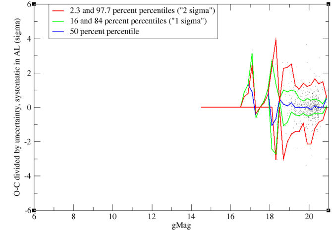
Lists 1 and 2 probably do not contain really truncated windows but were the result of VPU parameter adjustments (see Section 1.1.3). List 3 is probably the only list of transits with really truncated windows and contains less than 0.1 % of all transits. It is not the intention to give all the pictures for all the residuals for each of these lists. We just give as an example Figure 8.33, showing the SYST residuals in AL divided by their expected value for truncated windows of List 3. Note that the expected value of the residual does not depend on the fact whether the window is truncated or not. Since all truncated windows are fainter than magnitude 14, corresponding for a vast majority to 1D windows, AC residuals will not tell us anything interesting.
In List 3, the SYST residuals in AL are a bit larger than in the complete sample. But, apart from that, we see no significant difference between the AL residuals of the truncated windows and those of the complete list. Especially, in List 1, the RAND residuals follow rigourously the same distribution.
| gMag | 12 | 13 | 14 | 15 | 16 | 17 | 18 | 19 | 20 | total |
| C-03 | 0.0 | 0.0 | 1.4 | 0.6 | 11.5 | 7.0 | 8.8 | 11.4 | 11.0 | 10.7 |
| T-04 | 0.0 | 0.0 | 0.0 | 0.0 | 0.0 | 0.0 | 0.0 | 0.0 | 0.0 | 0.0 |
| C-05 | 0.0 | 0.0 | 0.0 | 0.0 | 0.0 | 0.0 | 0.0 | 0.0 | 0.0 | 0.0 |
| C-06 | 0.0 | 0.0 | 0.0 | 0.0 | 0.1 | 0.2 | 0.6 | 0.5 | 0.7 | 0.5 |
| C-07 | 0.0 | 0.0 | 0.0 | 0.0 | 0.0 | 0.0 | 0.0 | 0.0 | 0.1 | 0.0 |
| C-08 | 0.0 | 0.0 | 15.8 | 7.0 | 6.8 | 8.7 | 9.4 | 8.3 | 9.5 | 8.9 |
| C-09 | 34.6 | 16.7 | 32.7 | 17.3 | 10.9 | 18.3 | 20.4 | 15.2 | 14.4 | 15.6 |
| C-10 | 5.9 | 2.2 | 4.5 | 2.7 | 0.6 | 0.7 | 0.4 | 0.5 | 0.6 | 0.6 |
| T-11 | 0.0 | 0.0 | 1.6 | 0.0 | 0.0 | 0.2 | 0.0 | 0.1 | 0.1 | 0.1 |
| T-12 | 0.0 | 0.0 | 0.0 | 0.0 | 0.4 | 0.0 | 0.0 | 0.0 | 0.1 | 0.0 |
| T-13 | 0.0 | 0.0 | 0.5 | 0.0 | 0.9 | 0.2 | 0.5 | 0.8 | 0.7 | 0.7 |
| Total | 38.5 | 18.5 | 47.7 | 25.6 | 28.0 | 31.5 | 35.3 | 32.4 | 32.5 | 32.7 |
Table 8.15 gives, per magnitude bin, the performance of each position-based filter. Comparison with Table 8.12 shows that most filters behave in the same way for the truncated windows as for the non-truncated windows, with, however, one major exception, filter C-09. It shows a clear correlation between the presence of transits marked as having truncated windows and poor attitude.
The conclusion from this analysis is that there is no good reason to reject truncated windows.
Motions derived from single transits
Another way to assess the quality of the positions is to compare the motions of the SSOs as derived from the fit of a linear motion to the positions of single transits to those from a priori ephemerides. These ephemerides are derived from observations spread over many years, and hence motions from ephemerides will be much more accurate than motions derived from a single transit spanning only about 40 s, even if these positions are individually of much higher accuracy than those used for the ephemerides. In what follows, we assume that there is no error in the motions from the ephemerides, and that all differences between the motions from the ephemerides and those from the Gaia observations reflect the errors and the uncertainties of the Gaia observations.
From the uncertainties on the individual positions, one can derive a theoretical uncertainty in the motions. These uncertainties are computed as follows. Let be the epoch of position of the transit, the corresponding position as a vector with two components, AL and AC, the weight matrix of the position, i.e., the inverse of the covariance matrix of the random uncertainty (systematic errors do not influence the derived motion of an object), the square of the inverse of the uncertainty on the timing, which is supposed to be the same for all timings, the summation over all positions of the transit that have not been removed by any of the filters, and let Tr be the trace of the matrix. Compute as follows:
| (8.30) | ||||
| (8.31) | ||||
| (8.32) | ||||
| (8.33) | ||||
| (8.34) | ||||
| (8.35) | ||||
| (8.36) | ||||
| (8.37) | ||||
| (8.38) |
Then, is the motion of the SSO derived from the fit of a linear motion to the positions, and is its covariance matrix. In an (AL, AC) coordinate system, there is no correlation between the AL and AC motions, so that we can take the square root of its diagonal elements to get the uncertainties.
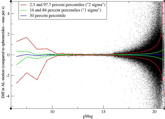
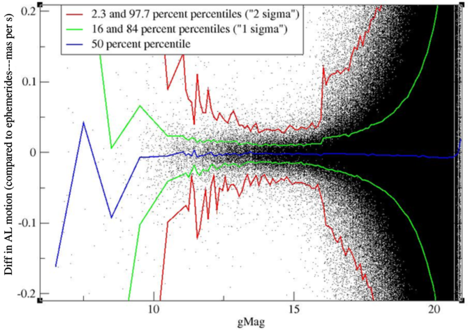
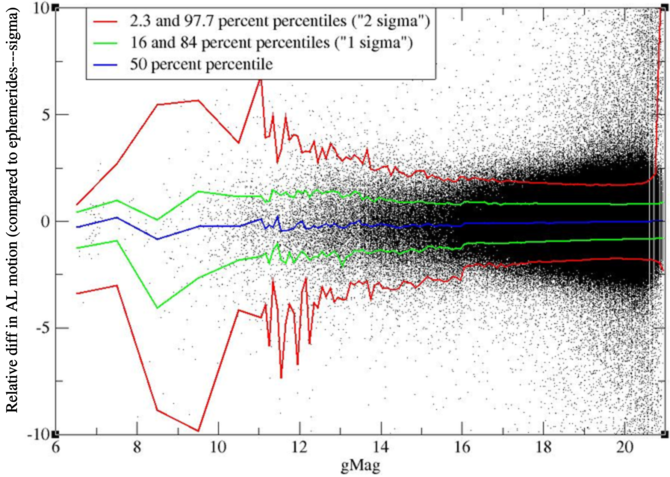
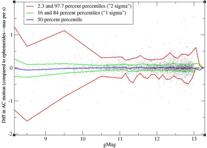
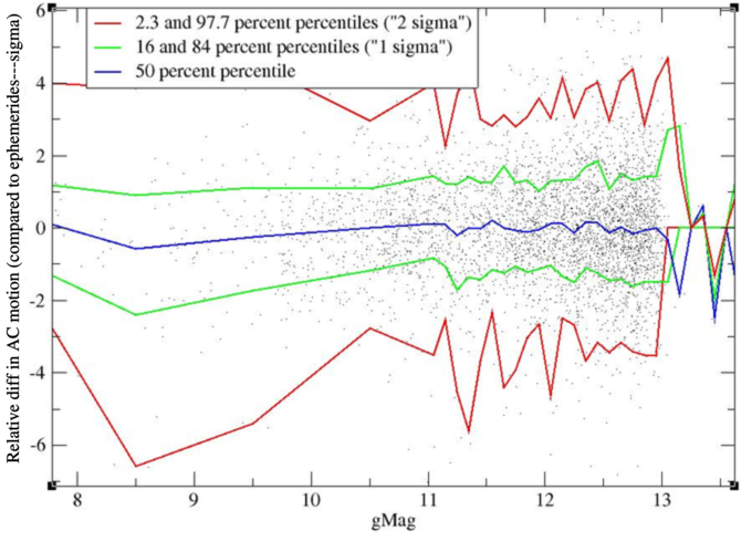
Figure 8.34 and Figure 8.35 show the difference between the motion derived in the astrometric reduction and the motion from the ephemerides as a function of magnitude. The motion is in milliarcseconds per second (mas s) . Note that typical values for the motion of an SSO observed by Gaia are of the order of 0–10 mas s. Quite expected, we find a minimum around magnitude 14 with differences of the order of 0.01 mas s. There is no more systematic offset, except that for very faint objects there is a systematic offset of only 0.008 mas s, which is really small.
Figure 8.36 shows the same difference in motion in AL divided by its computed uncertainty as given by Equation 8.38. We see that the behaviour of the difference is close to the expected behaviour, where for faint objects the difference is a bit smaller than expected and for bright objects a bit larger, but overall there is a rather good agreement with the expectations, and the asymmetry that was present in previous studies, has disappeared. It is thought that this is thanks to the application of the correct geometric calibration, as explained in Subsection 8.3.3.
The same exercise can be done in AC, but only for 2D windows. This is given in Figure 8.37 for the absolute difference and in Figure 8.38 for the relative difference. The figures are restricted to the magnitude range 8–13, because outside this range there are not enough transits with 2D windows to do the statistics. Results are comparable to those in AL.