8.4.4 Validation of Photometry
Author(s): Alberto Cellino, Laurent Galluccio, Karri Muinonen
SSO photometric data and principles of data validation
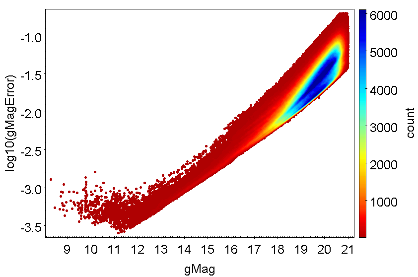
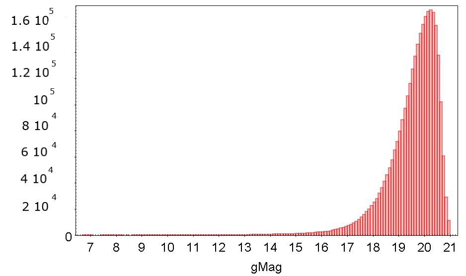
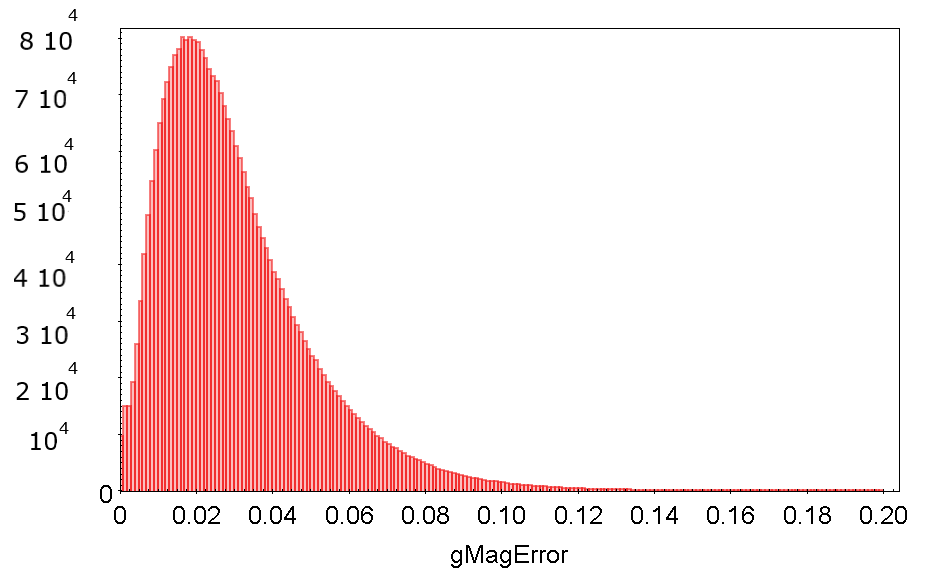
Figure 8.39 shows a plot of the error of apparent SSO magnitude (in logarithmic scale) as a function of for transits of SSOs selected for Gaia DR3. This plot shows the excellent quality of Gaia photometric data for SSOs. In spite of the apparent motion of these objects in the FOV, the typical photometric error is better than 0.01 mag for values up to mag.
Figure 8.40 and Figure 8.41 show the distributions of apparent magnitudes and associated errors for the same SSO transits selected for Gaia DR3. This catalogue of SSO transits has been produced after an extensive analysis of Gaia DR3 data. As explained in Section 8.3.5, the SSO photometric database was created starting from the SSO photometric fluxes computed by the PhotPipe system (see Chapter 5), and applying a further filtering based on the identification of problematic transits, according to the results of SSO astrometric data reduction (see Section 8.4.2). After that, all remaining SSO transits for which mag or the nominal error of was 0.2 mag were also removed. An additional filter to remove a relatively small number of transits (about 3700) for which the -magnitude nominal error turned out to be distinctly higher than normal, was also applied. Based on the experience achieved in analysing previous versions of the DR3 photometric dataset for SSOs, these transits had been already identified as being affected by errors due to a variety of problems. Figure 8.42 shows the resulting number of accepted SSO transits per object according to the adopted criteria. Note that, in spite of the large number of asteroids for which more than 20 or 30 transits are available, as shown in Figure 8.42, Figure 8.41 shows that only a fraction of these transits have nominal error bars sufficiently small to be conveniently used for validation purposes, in particular for photometric inversion techniques, as explained in Section 8.4.4 and Section 8.4.4.
To activate the procedures of data validation generally mentioned here and described, in more detail, in Section 8.4.4 and Section 8.4.4, ancillary information is needed for each transit, including the epoch in JD, the ecliptic coordinates of the object, the distance from the Sun and from Gaia, and the phase angle (see Section 8.4.4). This information, produced in advance by a simulation of the Gaia scanning law and on the available orbital information about SSOs, was available for transits.
How to assess that a dataset of photometric measurements of small SSOs is reliable? This is a complicated task, because each single photometric measurement of a small Solar System body like an asteroid is a unique and non-repeatable event. This is due to the fact that the brightness of an SSO measured at any given epoch depends on the observing circumstances, which vary with time over shorter and longer timescales and make any photometric measurement of an asteroid an event that is in practice non-repeatable.
In addition to time-dependent parameters, the measured brightness of an SSO observed at any given epoch depends also upon a set of constant physical parameters of the object, including the orientation of the spin axis on the celestial sphere (the pole of the object), the shape, the spin period, and the light-scattering properties of the surface.
Based on the considerations above, the validation of sparse SSO photometric measurements is not straightforward. It is based on two basic tools, namely an analysis of the phase-magnitude dependence of SSOs presented in the Gaia DR3 catalogue, as explained in Section 8.4.4, and on an analysis of the results of inversion tests for sparse photometric data, as explained in Section 8.4.4 and Section 8.4.4. The procedures and results described in the above mentioned sections represent a generalization and extension of procedures already adopted in the validation of Gaia DR2 data. In the case of DR3, however, the available data are better, both quantitatively and qualitatively, as will be explained.
Analysis of phase-magnitude data
A key parameter to describe the illumination conditions at the epoch of the observation of an SSO is the phase angle, the angle between the directions to the Sun and to the observer, as seen from the SSO. The phase angle is zero when the SSO is observed in conditions of ideal solar opposition (or in conjunction with the Sun, when the SSO is evidently not observable), and it reaches an upper limit that depends upon the orbit of the object and of the observer. Most distant SSOs can be observed from the Earth, or from the Gaia orbit, only in a narrow interval of possible phase angles, whereas objects approaching or sweeping the inner Solar System can be observed over a much wider interval of phase angles.
It is crucial to understand, however, that, as a consequence of the scanning law of Gaia, only very distant Solar System objects can be seen not far from solar opposition whereas, in the case of main-belt asteroids, the interval of possible phase angles starts from a minimum value of about and reaches a maximum value of about .
For the purposes of photometric validation, a crucial property of SSOs is that they tend to become fainter when observed at increasingly large phase angles. In the domain of phase angles covered by the Gaia observations, the behaviour consists of a nearly-linear increase of magnitude (normalized to unit distance) for increasing phase angle. It is therefore useful, as a first preliminary check of the Gaia asteroid photometry, to analyse the phase-magnitude relation.
 |
 |
 |
 |
 |
 |
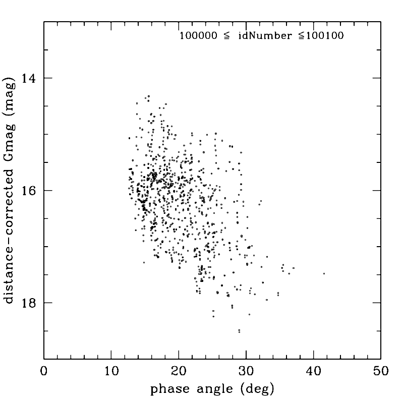
Figure 8.43 and Figure 8.44 display the phase-magnitude relation (-magnitude phase curve) for different subsamples of the asteroid transits recorded in Gaia DR3. They correspond to subsets of 100 objects exhibiting increasingly fainter magnitudes. These magnitudes were computed after a preliminary conversion of apparent magnitudes into the values corresponding to unit distance from both the Sun and Gaia. A generally encouraging linear trend of increasing magnitude for increasing phase angle is seen as expected, but the overlapping of data referring to different objects makes quantitative assessment difficult.
 |
 |
 |
 |
 |
 |
 |
 |
 |
 |
 |
 |
A more detailed analysis of the individual behaviour for large numbers of objects is then necessary. In the case of Gaia data, we deal with sparse measurements taken during a considerable interval of time. The phase-magnitude relation derived by such data is intrinsically noisy, because it includes measurements taken at epochs corresponding to different illuminated cross sections, due to both differences of rotation around the spin axis and the orientation of the body with respect to the line of sight, if data are taken at epochs sufficiently distant in time. In other words, the phase-magnitude curves shown in the DR3 database are contaminated by magnitude variations that are not uniquely due to differences in phase angle. In a phase-magnitude plot, this produces a decrease of data correlation.
This problem can be partially overcome if we consider the statistical behaviour of a large number of objects, something that is made possible by exploiting the fairly large Gaia DR3 database.
Some choices were made in order to mitigate the noise due to sparse photometry. First, for each object, among all the subsets of magnitudes measured during the same Julian day, generally corresponding to two or more consecutive detections in the two FOVs of Gaia, only the brightest recorded magnitude was kept for the analysis, to limit the noise due uniquely to different angles of rotation of the object around its spin axis. This was done to partly mimic the procedures used to analyse full lightcurves taken from the ground. Transits for which the measured magnitude had a nominal error of 0.05 mag or larger were discarded a priori. The next step was to discard all objects for which the interval of phase angles covered by the observations was narrower than . To ensure a reasonable sampling of the phase angle in the case of a larger number of available measurements, we discarded asteroids for which the number of magnitude measurements (after removal of all but one measurement taken during the same Julian day) was less than a limit related to the range of phase angles covered by the observations. This limit was chosen to be 4 if the covered range was larger than , 5 if the range was between and , and 7 if the range was between and . Finally, a linear least-squares fit of magnitude versus phase angle was computed.
After applying the filtering procedures described above, we computed for each considered asteroid a linear fit of its phase-magnitude relation. A statistical analysis of the behaviour of the results was done for two different sub-samples: the first includes asteroids numbered between 1 and 10 000. Among them, 9107 passed the filters described above, and were accepted for the computation of the best-fit linear slope. The second sample was chosen to be that of asteroids numbered between 100 000 and 110 000. Among them, 4802 were accepted for a phase-magnitude analysis. The decrease of the number of accepted asteroids in different regimes is related to the decreasing number of acceptable transits for increasing faintness. The two samples allow us to compare the phase-magnitude behaviour of objects in two distinct magnitude regimes. Some results of this statistical analysis are shown in figures from Figure 8.45 to Figure 8.50, displaying some general properties of the two considered samples.
These figures include the histograms of some parameters of fundamental importance for the analysis, namely the number of magnitude measurements per object and the range of phase angles covered by the observations of each object. The distribution of the computed linear slopes and the distribution of the corresponding formal errors are also shown, as well as the distribution of the correlation of phase-magnitude data used in the analysis. The distribution of computed linear slopes tends to peak around reasonable values. The existence of a small fraction of aberrant cases of objects exhibiting negative slopes (corresponding to objects for which the brightness seems to increase for increasing phase angle) cannot be over-emphasized, taking into account the possible problems coming from still small number of measurements per object, distributed over an interval of epochs possibly corresponding in some cases to quite different observing circumstances. The plots show that the vast majority of objects exhibits values of the slope that correspond to general expectations, taking also into account some expected differences depending on the surface properties of different taxonomic classes of objects.
The general results of this analysis of DR3 SSO data indicate that, in the vast majority of cases, reasonably good linear fits of the phase-magnitude relation are obtained, with slopes which are compatible with those that are typically obtained from ground-based measurements. The latter are based on full lightcurves obtained over limited intervals of time in which the most important change of observing circumstances is given by differences in phase angle only. In the case of the sparse Gaia photometric data available in DR3, some aberrant results are found, but the number of these cases is small and can be minimized by simply imposing tighter acceptance criteria in terms of input data quality (number of observations and covered interval of phase angle). By adopting more conservative acceptance criteria for the computation of linear fits of available phase-magnitude data, it is possible to obtain a nearly total removal of the cases of negative slope values.
Some tests of photometric inversion
For the purposes of validation of Gaia DR2 SSO photometric data, some important tests relied on a comparison of measured versus predicted magnitudes for small sets of observations of the same object obtained at different epochs. Now, taking advantage of the much larger amount of SSO photometric data available in Gaia DR3, a more systematic attempt of full photometric inversion has become possible. This means that the available data can be sufficient to carry out an attempt at inferring the values of the spin, shape, and light-scattering parameters that are responsible of the measured photometric behaviour.
Using magnitudes reduced to unit distance, one can analyse the variation of the intrinsic brightness of any given object measured at different epochs. Having a set of sparse photometric measurements of the same object, it is convenient to work in terms of brightness differences with respect to one of the available measurements (usually, the first measurement). In this way, any dependence upon constant light-scattering properties of the surface can be removed, assuming that the surface has homogeneous properties. This reduces the time-dependence of the measured brightness data to a function of the rotation period, overall shape, orientation of the spin axis, and dependence upon the illumination conditions, described in terms of the phase angle (see Section 8.4.4). A simple dependence upon the phase angle summarizes, for the sake of simplicity, the overall effect of the mechanisms of single and multiple scattering of sunlight incident onto the surface.
Based on the above considerations, it is possible in principle to develop algorithms which determine the unknown physical parameters of an object whose brightness has been measured by Gaia in a sufficiently large number of observed transits. In principle, the best possible validation test must consist of comparisons between the computed physical parameters and those already known for a set of objects for which our knowledge of their physical parameters is extraordinarily accurate, being based on in situ measurements carried out by space probes. The number of these objects, unfortunately, is still very small, and they deserve a separate treatment in Section 8.4.4.
In the vast majority of cases, we must base our analysis upon objects for which we have reasonably reliable estimates of the rotation period, pole, and shape based on available evidence coming from analyses of data, collected in the vast majority of cases from the ground. In most cases, such knowledge is based on the availability of good-quality photometric lightcurves.
Modern methods of photometric inversion allow the determination of sophisticated shape models described by many parameters. In the case of Gaia data, however, the need of treating very large numbers of objects, each one observed at tens of different epochs, obliges us to adopt a very simple shape model, namely a triaxial ellipsoid shape depending upon two parameters only, i.e., two axial ratios. This choice allowed us to use analytical relations to compute the expected brightness in any given observing circumstance, decreasing dramatically the needed computing time. As for our treatment of light-scattering effects, it is assumed that asteroid surfaces scatter incident sunlight according to a Lommel-Seeliger relation. The corresponding dependence of brightness upon phase angle for a triaxial ellipsoid asteroid has been resolved analytically (Muinonen and Lumme 2015). It is important to note that it is assumed that the optical properties of the surface of the object are homogeneous, and the photometric behaviour is essentially due to the shape of the object, seen in different configurations and illumination conditions at different epochs. This approach was implemented in our algorithm for photometric inversion of asteroid magnitude data.
The adopted numerical code for the inversion of sparse photometric data is based on a genetic algorithm, which carries out a search for the set of unknown parameters of a given object, minimizing the difference between a set of measured magnitudes and those corresponding to an object having a triaxial ellipsoid shape. The unknown parameters are seven: the spin period ; the pole ecliptic longitude and latitude; two axial ratios describing the triaxial ellipsoid shape; one parameter describing an assumed linear dependence of the brightness upon the phase angle; a value for the initial rotation angle of the object at the epoch of the reference observation epoch, chosen to be the first observation in chronological order. This algorithm was applied in the past to perform photometric inversion of data produced both by simulations (Santana-Ros et al. 2015) and by the Hipparcos satellite (Cellino et al. 2009). A most recent application, including an analysis of SSO data published in Gaia DR2, was published by Cellino et al. (2019).
Note also that a sign was assigned to each obtained solution, according to the IAU conventions. This means that the ecliptic latitude of the pole was always given as a positive value. In all cases in which the ecliptic latitude of the pole would turn out to be negative, meaning that the sense of rotation is opposite, the ecliptic latitude was set to its positive value, the ecliptic longitude of the pole was increased by , and the sign of the period was set to its negative value. This means that the obtained inversion solutions give also the sense of rotation of the objects.
In the validation tests, a large number of objects were considered, which have been the targets of remote observations from the ground. Decades of ground-based photometry, mostly at visible wavelengths, have produced large catalogues of asteroid lightcurves from which the rotation periods have been derived with good accuracy for a dataset of the order of 10 000 objects. Among them, a smaller number of objects have been observed in a variety of observation circumstances sufficient to derive for them accurate estimates of the spin axis direction. In many cases, more than one pole solution is found to be compatible with the available data. In a large number of cases, an overall shape, derived using complex algorithms of lightcurve inversion, has been also obtained. Shape details, however, are of limited importance in our case, because we compute photometric inversion using a simple triaxial ellipsoid shape which is only a first approximation of what can be the real shape of an asteroid. In our analysis, we used currently available catalogues of asteroid rotation periods and pole coordinates. In particular, we massively exploited the DAMIT (Database of Asteroid Models from Inversion Techniques), publicly available on the web at the URL https://astro.troja.mff.cuni.cz/projects/damit/. For objects not included in DAMIT, we took the periods from the Asteroid Lightcurve Data Base catalogue, available at the web site of the NASA Planetary Data System.
We limited our analysis to all asteroids numbered between 1 and 1000 for which at least 30 accepted transits are available in the Gaia DR3 database. In particular, we accepted only transits for which the nominal error of the magnitude is not larger than 0.02 mag, because the results of photometric inversion are negatively affected by using data of insufficient quality. Because the quality of Gaia photometry is excellent, in any case our sample of targets includes objects sufficiently bright to have magnitude uncertainties systematically smaller than the above limit. The resulting sample used for our photometric inversion test includes 430 asteroids.
It should be emphasized that the adopted inversion algorithm produces for each object a set of 15 different inversion solutions. In the results that are shown below only the solution giving the smallest residuals was taken into account. It is important to note, however, that in several cases more than one solution, among those that were obtained by the inversion algorithm, gave practically equal residuals, differing by no more than 0.0015 mag. In particular, there are cases in which the nominally best solution is not the one corresponding to the rotation period and pole listed in catalogues based on ground-based observations, whereas another equivalent solution would correspond to these values. It is planned to treat these ambiguous cases in the future by listing for each object all the equivalent best-fitting solutions. This was not done at this stage. Therefore, the results presented here are conservative, because we considered one solution per object, only.
It should be emphasized that, for the purposes of inversion of a set of sparse photometric measurements, the data should include measurements sampling adequately the whole interval of in ecliptic longitude. This is especially important for the determination of the pole. However, this is not yet the case for the data available in Gaia DR3. For each object, large gaps exist in the interval of covered ecliptic longitudes. Note also that the publication of photometric inversion of Gaia data is scheduled as an end-of-mission task. The results of the preliminary inversion attempts presented here must therefore be considered as no more than a useful tool for the scientific validation of Gaia DR3 data.
We classify as a successful determination of the rotation period an inversion solution for which
This criterion takes into account the fact that, for fast rotations, larger differences in lead to important differences in the rotational phase of the object computed at different epochs. On the other hand, in the case of long rotation periods, larger than several tens or hundreds of hours, it is not reasonable to impose a required accuracy of the order of few seconds in the determination of the period. Moreover, we can say that our criterion is intrinsically very severe, since it assumes that the values listed in the literature have always extremely small uncertainties. This can be true in most cases, but we should not forget that there can be objects for which a value from ground-based observations can be affected by significant uncertainty, in particular, when the period is longer than some tens of hours. By the way, long- objects are likely to be under-represented in currently available catalogues, due to the practical difficulties to obtain for them photometric data sufficient to derive a reliable rotation period. Based on our adopted criterion, taken at face value, we obtained the right period solution for 229 out of 430 asteroids in our sample.
 |
 |
In Figure 8.51, the left panel shows the absolute value of the difference of as a function of the value listed in the literature. The right panel of the figure shows the same, but here the difference is normalized to the value of listed in the literature (this corresponds to our abovementioned criterion to define a correct inversion solution for ). One can see that, as expected, the difference tends to increase for increasing , and that, for periods longer than about hours, our criterion for a successful inversion looks reasonable. Even more importantly, as shown more clearly in the right panel of Figure 8.51, there is a fairly large number of cases in which the value resulting from photometric inversion turns out to be nearly exactly twice the value listed in the literature. This fact is not unexpected, and there are two possible explanations. It is due to the assumed lightcurve morphology expected for an object having a triaxial ellipsoid shape. In some cases, the time sampling of the photometric variation can be unfavourable, and the resulting coming from photometric inversion can correspond to an object spinning with a period twice the real value. An alternative explanation, however, is more interesting. The inversion algorithm assumes that the object’s surface is homogeneous and the brightness variation for a triaxial ellipsoid shape includes two maxima and minima per rotation. However, there can be objects having important surface inhomogeneity (possibly due to craters excavating materials having different optical properties, as in the case of (4) Vesta). If the shapes of these objects are close to spheroids, their photometric variation will not be simply due to the shape, but will be dominated by local albedo heterogeneity, producing one maximum and one minimum only per rotation cycle. Due to the assumption of surface homogeneity and triaxial shape, the inversion algorithm will assign to these objects a period equal to twice the right value.
 |
 |
 |
 |
Summarizing, the results shown in Figure 8.51 look encouraging. The computed values are generally close to the values listed in the literature with the interesting existence of cases for which the computed value is twice the ground-based value. It will be interesting to see, whether the fraction of these cases will be confirmed in future Gaia data releases, when the number of high-quality photometric data points per object will increase significantly.
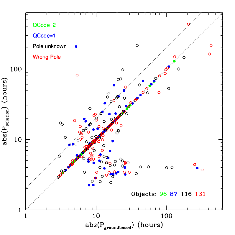
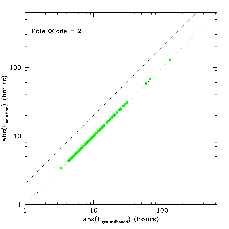
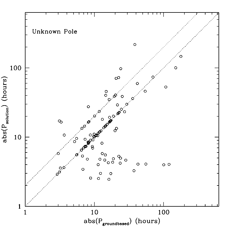
As for the pole, the situation is intrinsically more complicated. In the vast majority of cases, two or more different pole solutions per object are listed in the literature. Moreover, in our case of a triaxial ellipsoid shape model assumption, there is sometimes an ambiguity of in the determination of the ecliptic longitude of the pole, due to the symmetry of the shape model. The analysis was limited to a comparison of DAMIT asteroid poles, only, and it was decided to define a small number of Quality Codes (QCodes) to subdivide subjectively the obtained pole solutions. In particular, QCode = 2 was assigned to pole solutions differing by no more than about in (separately) ecliptic longitude and latitude with respect to one existing DAMIT pole solution, and imposing also that the rotation period determination was correct. QCode = 1 was assigned to inversion solutions for which the best pole solution was (subjectively) not so close to a DAMIT pole solution, but not very far from it, independently of the obtained period. A pole QCode = 1 was assigned to situations in which the obtained pole solution had little to do with any existing DAMIT solution. Finally, QCode = 0 was assigned to cases for which no DAMIT pole solution exists. Figure 8.52 shows a plot, in logarithmic scale, of the computed from inversion of Gaia DR3 photometric data and the value listed in literature for the objects of our sample. Different colours correspond to differently assigned QCodes. Note that in this plot, the objects for which the computed solution is twice the value found in the literature (see above) are clearly indicated, as well as those for which the computed is practically identical to the literature value.
The results of photometric inversion analysis indicate that, as expected, a correct inversion in terms of rotation period determination does not correspond necessarily to a correct pole solution, and vice versa. This is due to the still insufficient coverage of the ecliptic longitude range by the Gaia DR3 observations, as mentioned above. Some inversion failures can certainly be due to the use of a simplistic shape model. The good percentage of successful period determinations should not be underappreciated, however, considering both the limits of the adopted shape model, and the fact that correct solutions producing equivalent RMS residuals have not been taken into account in the analysis for the moment.
Although this photometric inversion test was limited to a relatively small sample of relatively bright objects, the results obtained can be interpreted as an overall confirmation of the good quality of the Gaia DR3 SSO magnitudes. Extending the inversion analysis to much fainter asteroids would not produce very useful results due to the lack of ground-based comparison. Ground-based period and pole solutions are rare for faint objects. In this respect, however, we should mention that a few dedicated tests led to correct inversion solutions, according to literature data, for a few asteroids numbered above 100 000.
Coupled with the results of the analysis of the phase-magnitude relation, the results described in this Section indicate that the Gaia DR3 SSO magnitudes are of good quality.
| (21) Lutetia | (2867) Šteins | |
| 8.168270(1) | 6.04681(2) | |
| , | 52.2(4), 7.8(4) | I: 96(5), -85(5) |
| II: 142(5), -83(5) | ||
| Class | M | E |
 |
 |


Tests on objects observed in situ
The present validation consists of comparing the observed Gaia photometry to photometry computed for known asteroids that have accurately determined rotation periods, pole orientations, and high-resolution shape models. In Gaia DR3, there are photometric data for more than a dozen asteroids studied by space missions. By using the shape models, rotational parameters, and taxonomical classifications of (21) Lutetia and (2867) Šteins, asteroids visited by the ESA Rosetta space mission, we study if it is possible to validate the Gaia DR3 SSO photometry. We note that (21) Lutetia and (2867) Šteins were assessed earlier in the documentation of Gaia DR2.
For (21) Lutetia and (2867) Šteins, the Planetary Data System provides the shape models illustrated in Figure 8.55 as well as the rotation periods and pole orientations described in Table 8.16 (Farnham and Jorda 2013; Jorda et al. 2012; Farnham 2013; Sierks et al. 2011). The table also includes the Tholen taxonomical classes of the two asteroids.
The Gaia DR3 photometric measurements for these two asteroids are plotted as a function of the epochs of observation, expressed in days after the first observation, and against the phase angle in degrees, in Figure 8.56. Both phase-magnitude relations show a decreasing trend in disk-integrated brightness with increasing phase angle. Furthermore, the apparent slope of decreasing brightness is steeper for Lutetia, in agreement with Lutetia and Šteins being lower-albedo M-type and higher-albedo E-type objects in the Tholen taxonomy, respectively.


 |
 |
The study on (21) Lutetia with the 23 transit magnitudes obtained by Gaia was started (Case I) by using a shape model derived from combined ground-based relative photometry and Gaia photometry with convex inversion methods (Muinonen et al. 2020; Kaasalainen et al. 2001). The results showed that the Gaia measurements contributed to the shape modelling with reasonable residuals, with an RMS value of 0.022 mag (see Figure 8.57). Next (Case II), it was seen that using the best available shape model (Farnham 2013), constructed by combining together a high-resolution shape model based on disk-resolved imaging by Rosetta and a lower-resolution model based on ground-based relative photometry and silhouette observations with adaptive optics, it was not possible to produce a straightforward fit to the Gaia observations. By optimizing the rotational phase of Lutetia and the slope of the phase curve implied by the Lommel-Seeliger scattering model, the high-resolution shape model reproduced the Gaia photometry with a large RMS value of 0.046 mag. We interpreted this as a strong indication that the Gaia data offers new information on the shape and modifies the currently accepted shape solution.
A closer inspection of the time distribution of the 23 transit magnitudes shows that, for 12 of them, Lutetia’s hemisphere predominantly visible to Gaia was that not mapped by Rosetta. It is therefore highly probable that the Gaia data provide additional information on that portion of the asteroid surface. In particular, the Gaia photometry, with its absolute phase angle dependence, relates the sizes and geometric albedo characteristics of the two hemispheres.
We modelled directly, by using the high-resolution shape, the photometry of the remaining 11 observations, obtained with the hemisphere mapped by Rosetta in view (Case III). Allowing for optimization in only the rotational phase and the slope of the phase curve implied by the Lommel-Seeliger scattering model, the high-resolution shape model reproduced the Gaia photometry with an excellent RMS value of 0.016 mag. We then applied an analogous approach to the 12 observations obtained with the hemisphere not mapped by Rosetta (Case IV). With constant geometric albedo characteristics, the RMS value was large at 0.053 mag.
The photometric slopes implied by the Lommel-Seeliger scattering model were in excellent mutual agreement in all Cases I-IV studied above. In the cases of convex optimization using all Gaia DR3 measurements (Case I), optimization of the rotational phase and slope using the high-resolution shape model and all Gaia DR3 measurements (II), measurements corresponding to the hemipshere observed by Rosetta (III), and measurements corresponding to the hemisphere not observed by Rosetta (IV), the slopes were, respectively, 1.52 mag rad, 1.56 mag rad, 1.60 mag rad, and 1.58 mag rad. Based on Penttilä et al. (2016), Muinonen et al. (2020), and Martikainen et al. (2021), the values correspond to slopes of Tholen S-class and M-class asteroids.
We conclude that Gaia photometry is probably better than 0.01-0.02 mag, but the limitations on, first, the shape model accuracy does not allow us to push the analysis further. Second, we are assuming the same Lommel-Seeliger scattering model to be valid everywhere on the surface of Lutetia. In particular, we are assuming that a single combination of geometric albedo and scattering phase function is representative of the entire surface of Lutetia. Third, it is not possible to exclude that some anomalous brightness values are present.
The results obtained for (2867) Šteins, whose high-resolution shape model does not suffer from hemisphere-scale limitations similar to those of (21) Lutetia, support the idea that Gaia photometry is indeed accurate. In the case of this object, there are two pole solutions (Cases I-II, see Table 8.16), differing, essentially, only in terms of the zero point of the rotational phase. By directly using the shape model to reproduce the Gaia data, re-sampled at a 5-degree resolution, the RMS values of the Observed-Computed magnitudes turn out to be 0.019 mag and 0.021 mag for the two pole solutions. These fits are based on 30 photometric points of which 3 had to be omitted as outliers. Using the same treatment as in the case of Lutetia, the fits were obtained by optimizing only the rotational phase and the photometric slope implied by the Lommel-Seeliger scattering model. For both pole orientations, the photometric slope obtained values of 1.47 mag rad (Case I) and 1.50 mag rad (II), realistic for high-albedo E-class asteroids (Penttilä et al. 2016; Muinonen et al. 2020; Martikainen et al. 2021). Considering the simplicity of the surface scattering modelling utilized, this is a good result depicted in Figure 8.58. The remaining limitations, in the case of (2867) Šteins, are still related to details of the shape model and surface scattering characteristics. In particular, certain assumptions were made on the scattering properties, when the high-resolution shape model was derived from the Rosetta images. It remains possible that the three observations omitted as outliers were omitted due to modelling issues rather than low observational accuracy.
In conclusion, our validation shows that Gaia epoch photometry, appropriately filtered to eliminate the outliers, has probably an accuracy better than 0.01-0.02 mag. We cannot rule out, however, the possibility that the sample published in Gaia DR3 could still include a non-negligible fraction of anomalous data. We recommend detailed analyses and careful verifications in applying the Gaia DR3 photometry of asteroids.