7.2.7 Quality assessment and validation

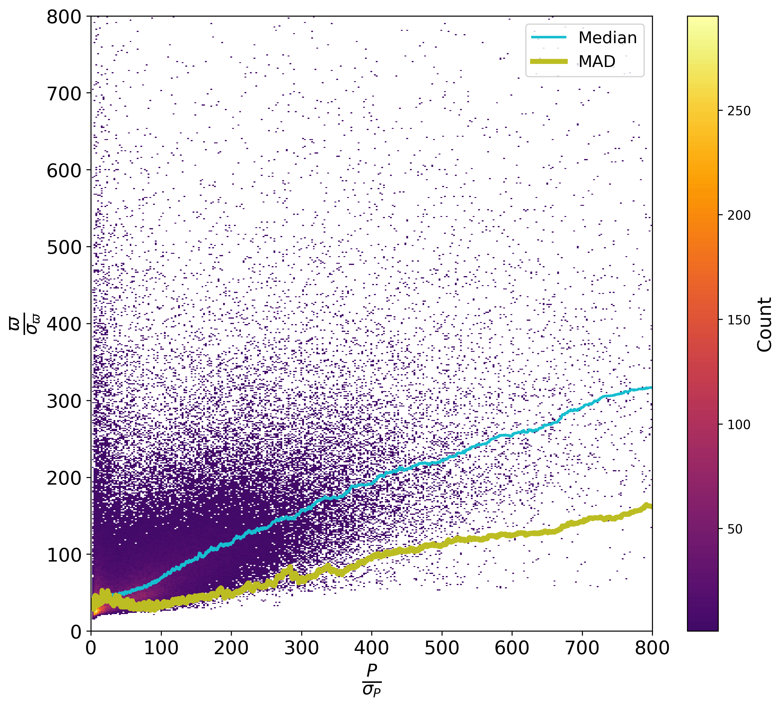
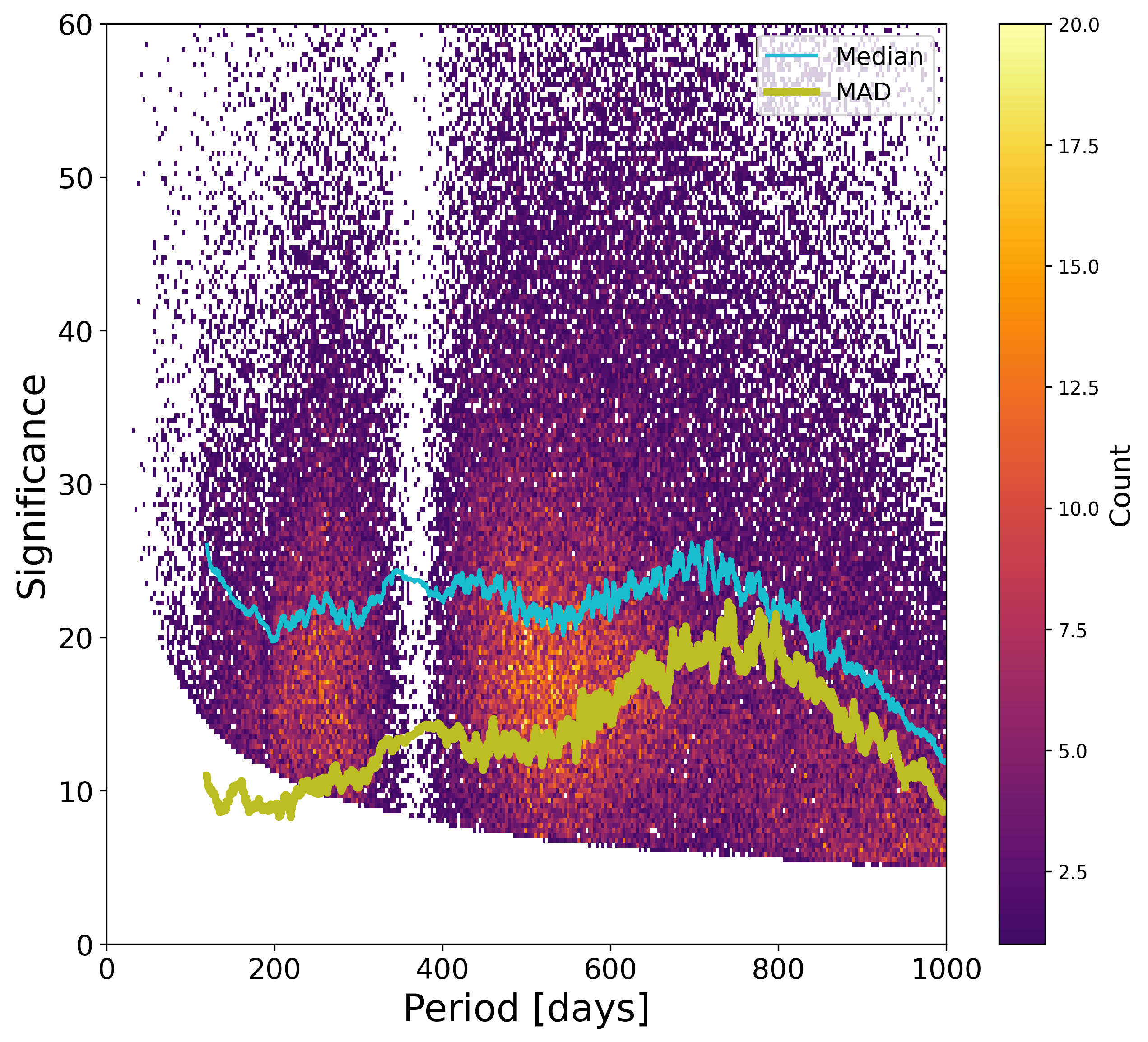
The observed distribution of the parameters obtained by the NSS processing is the convolution of the true distribution in our Galaxy with the full processing chain, and its selection effects, whether voluntary or not. Of particular importance is the effect in practice of the internal filtering which allowed to dismiss many wrong solutions. The truncations applied of some parameters of the orbital solutions can be seen in Figure 7.10, concerning period, parallax S/N, significance. In these and the following plots, a running median and running median absolute deviation (MAD) over 1 000 points have been as robust estimates of the centre and dispersion of the distributions respectively. Note that the MAD has not been normalised here so that it is expected to be $\sim 0.67$ for a Gaussian distribution of unit variance and $\sim 0.25$ for a uniform distribution.

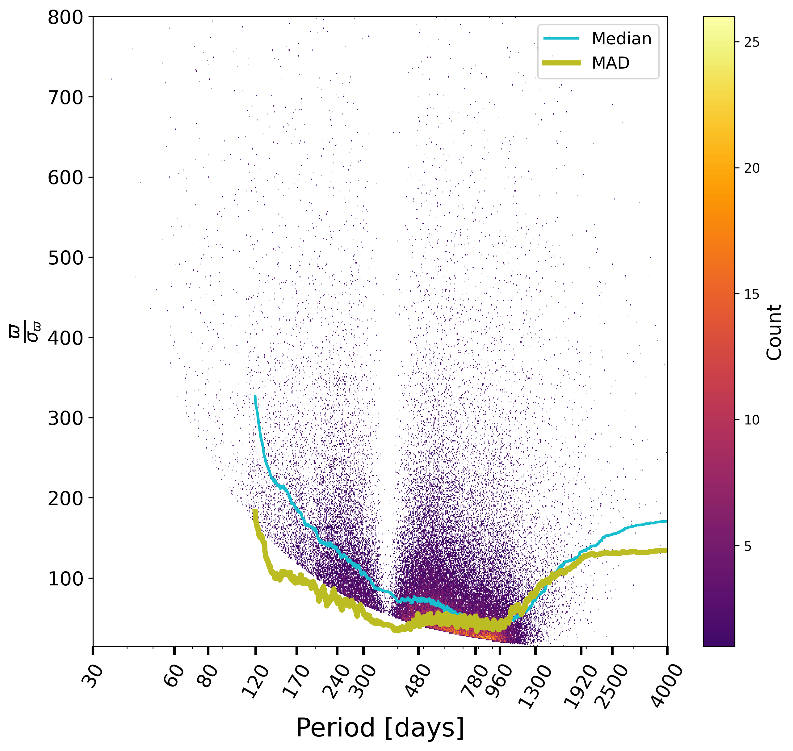
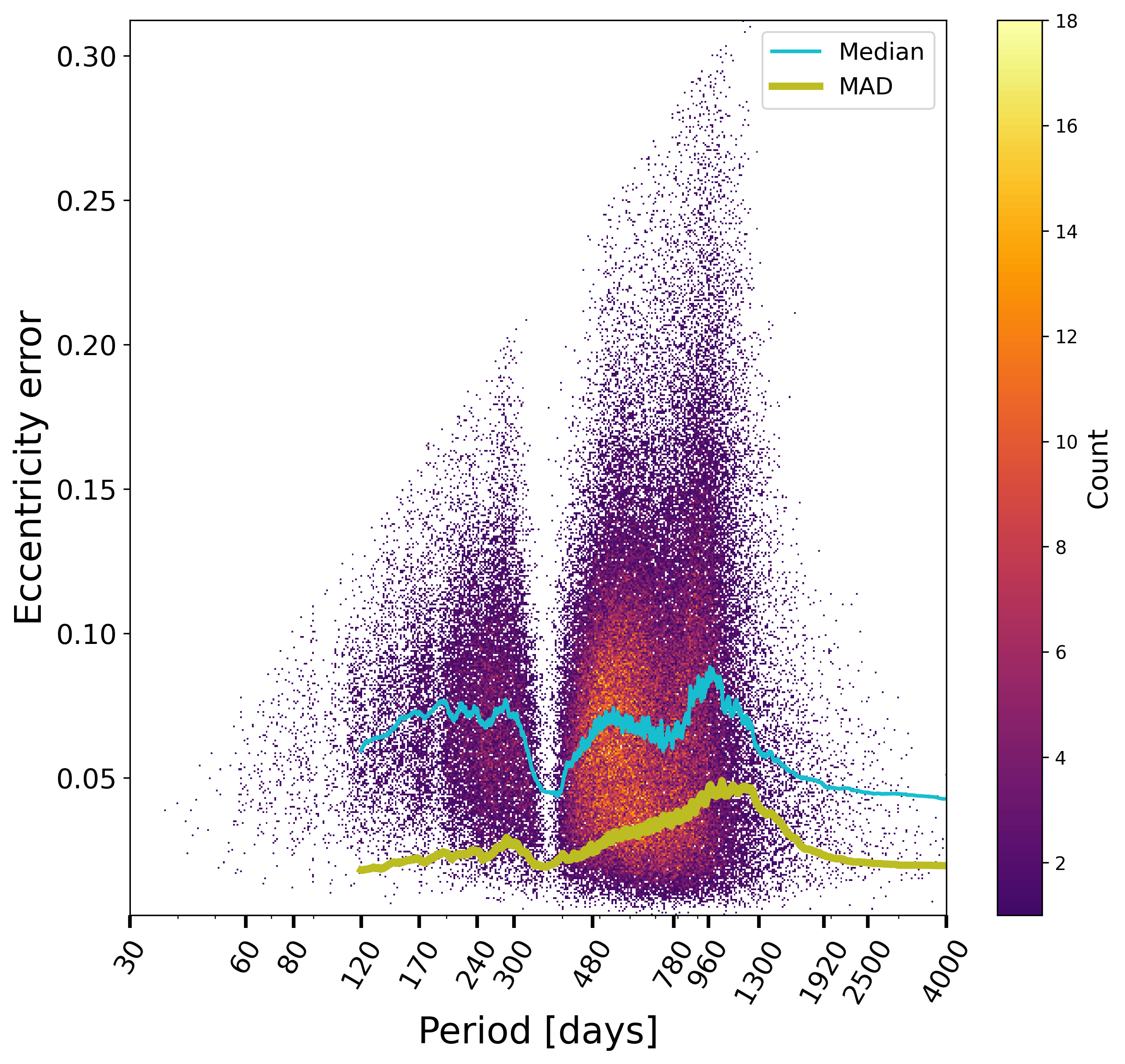
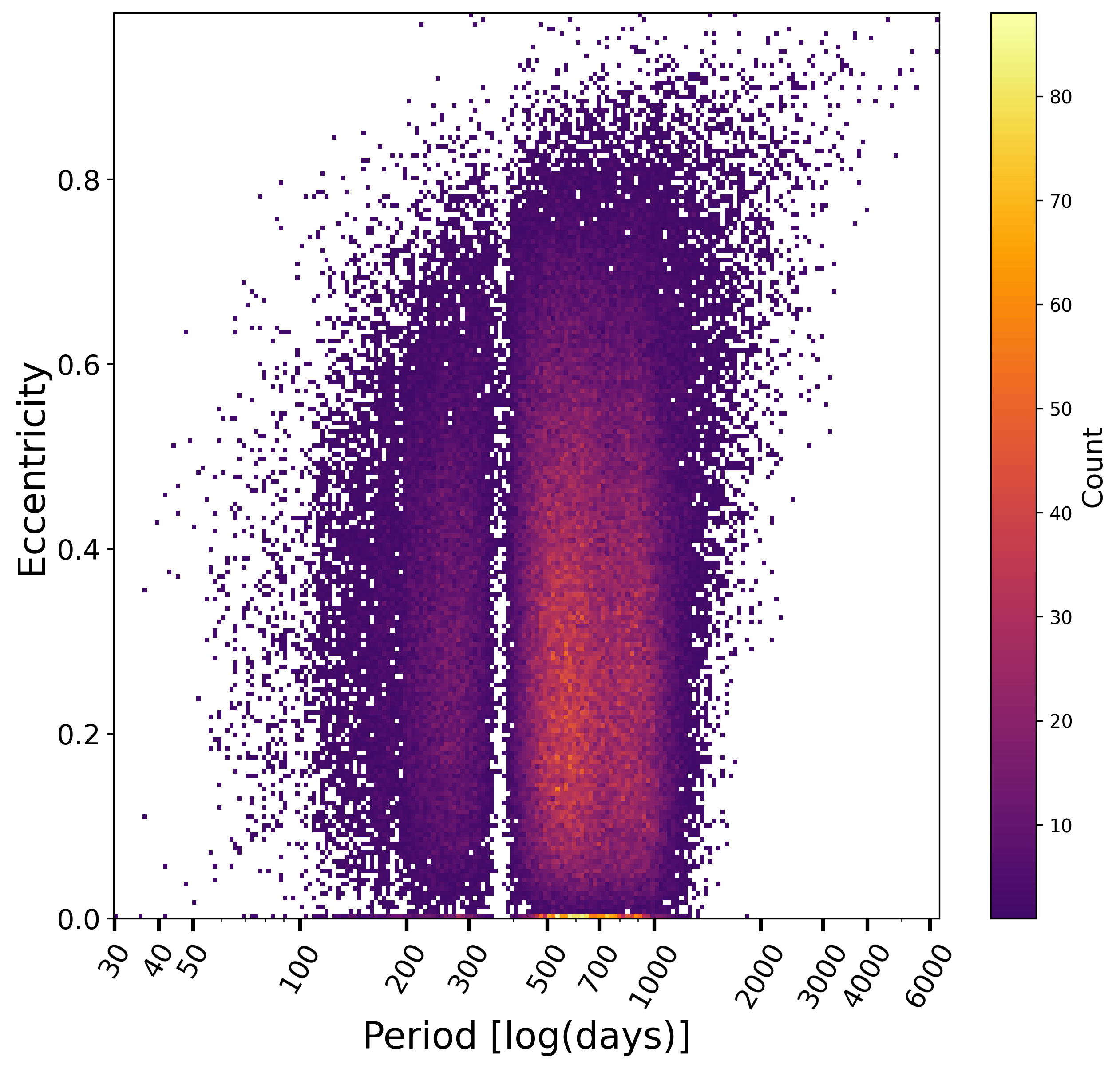
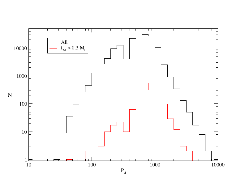
The period-eccentricity relation for the retained solutions, Figure 7.11a, looks as expected, with its circularisation effect, and the conspicuous lack of solutions around one year period, also seen in Figure 7.10, due to the impossibility to decouple the orbit from the parallactic effect. The distribution of periods, Figure 7.11b, also shows that the rate of large mass functions is larger at long periods, also expected.

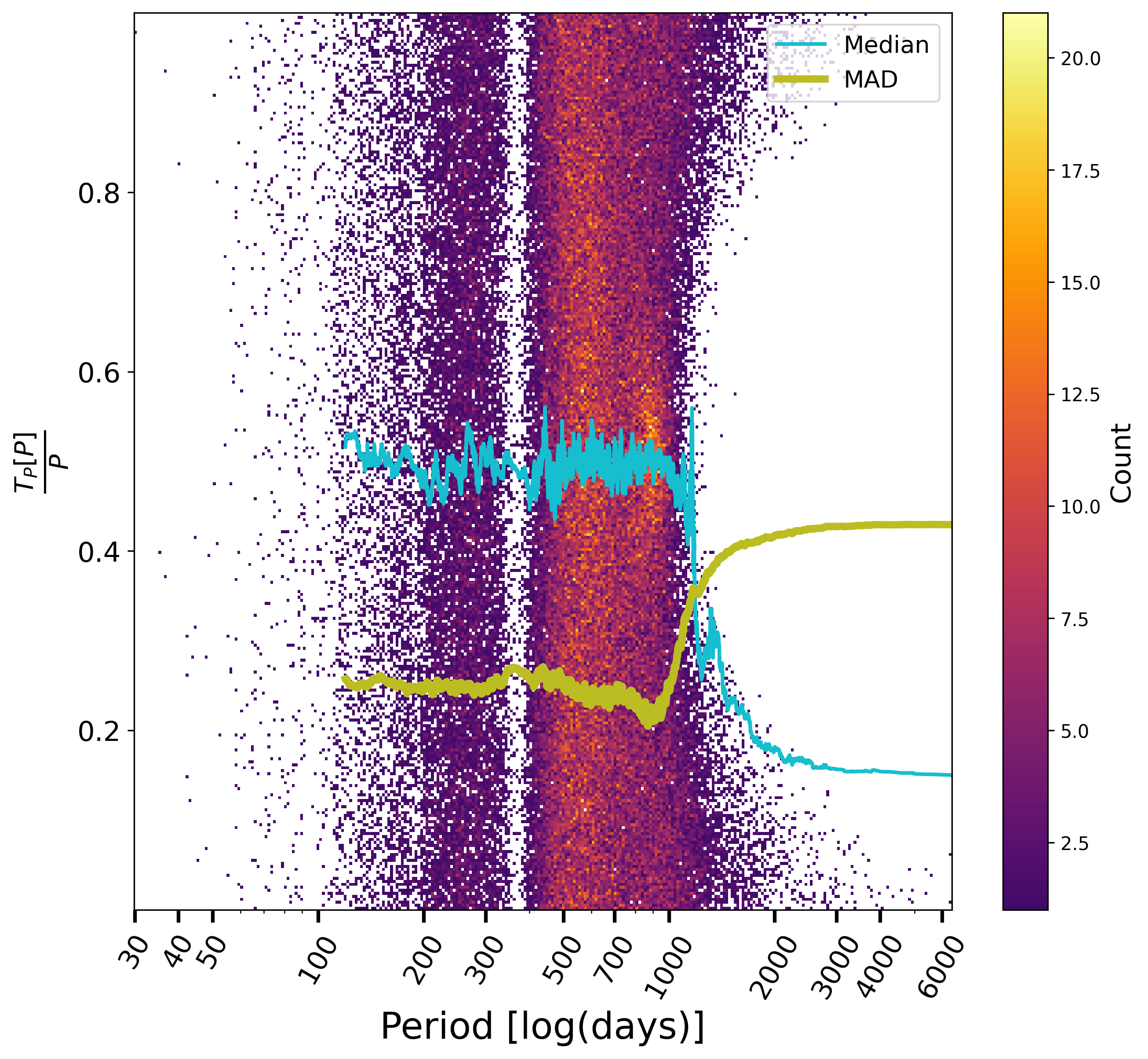
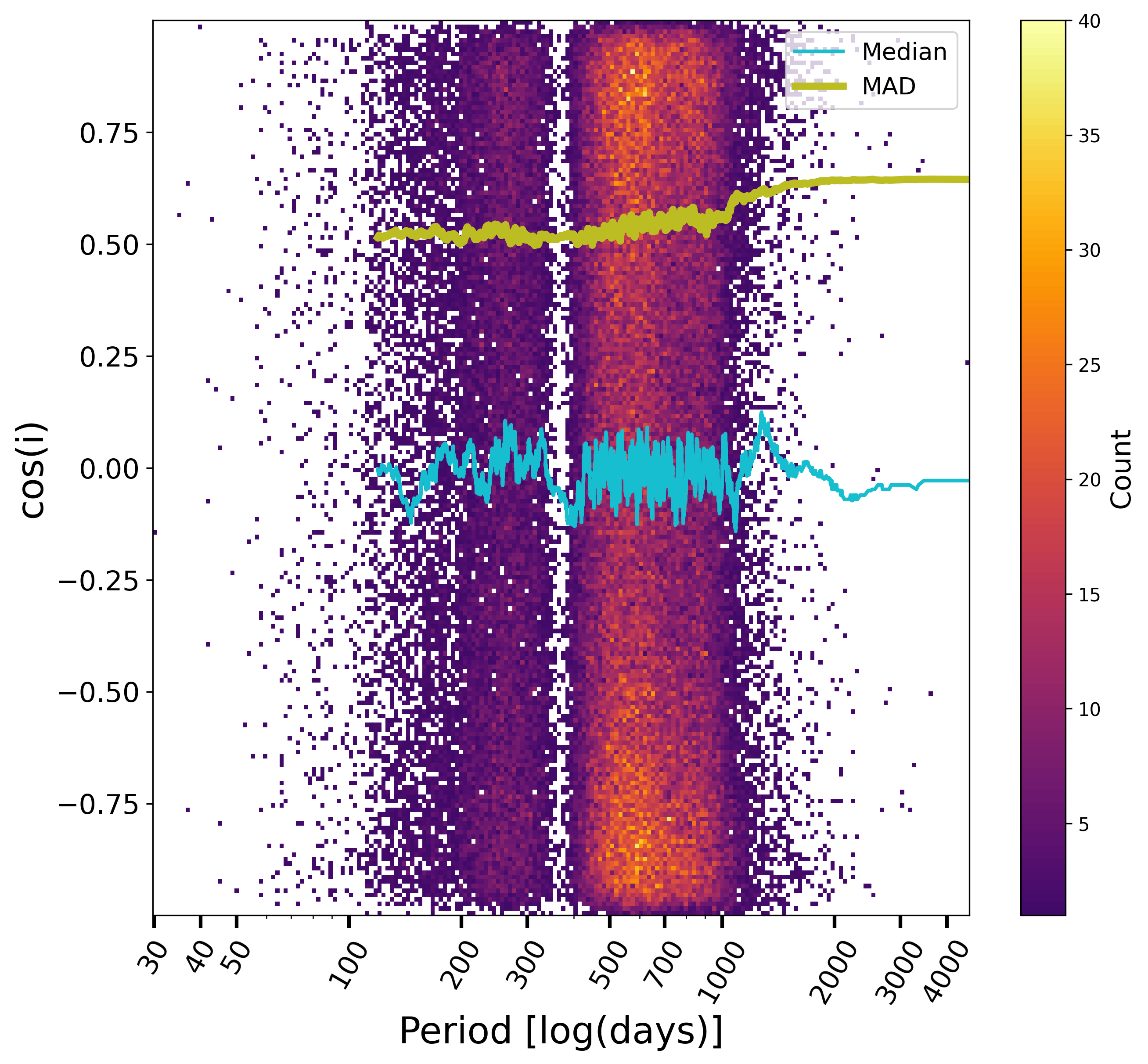
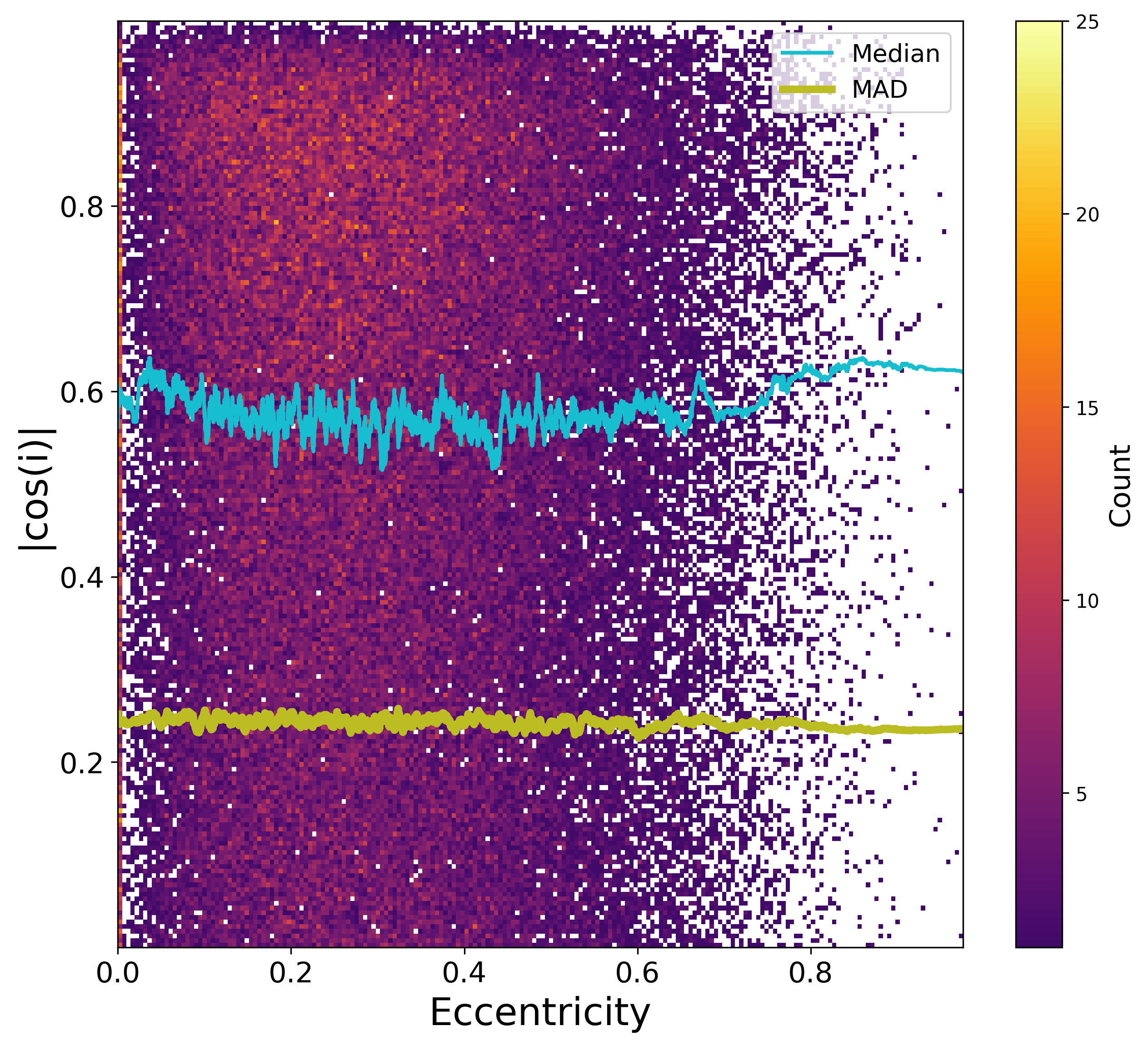
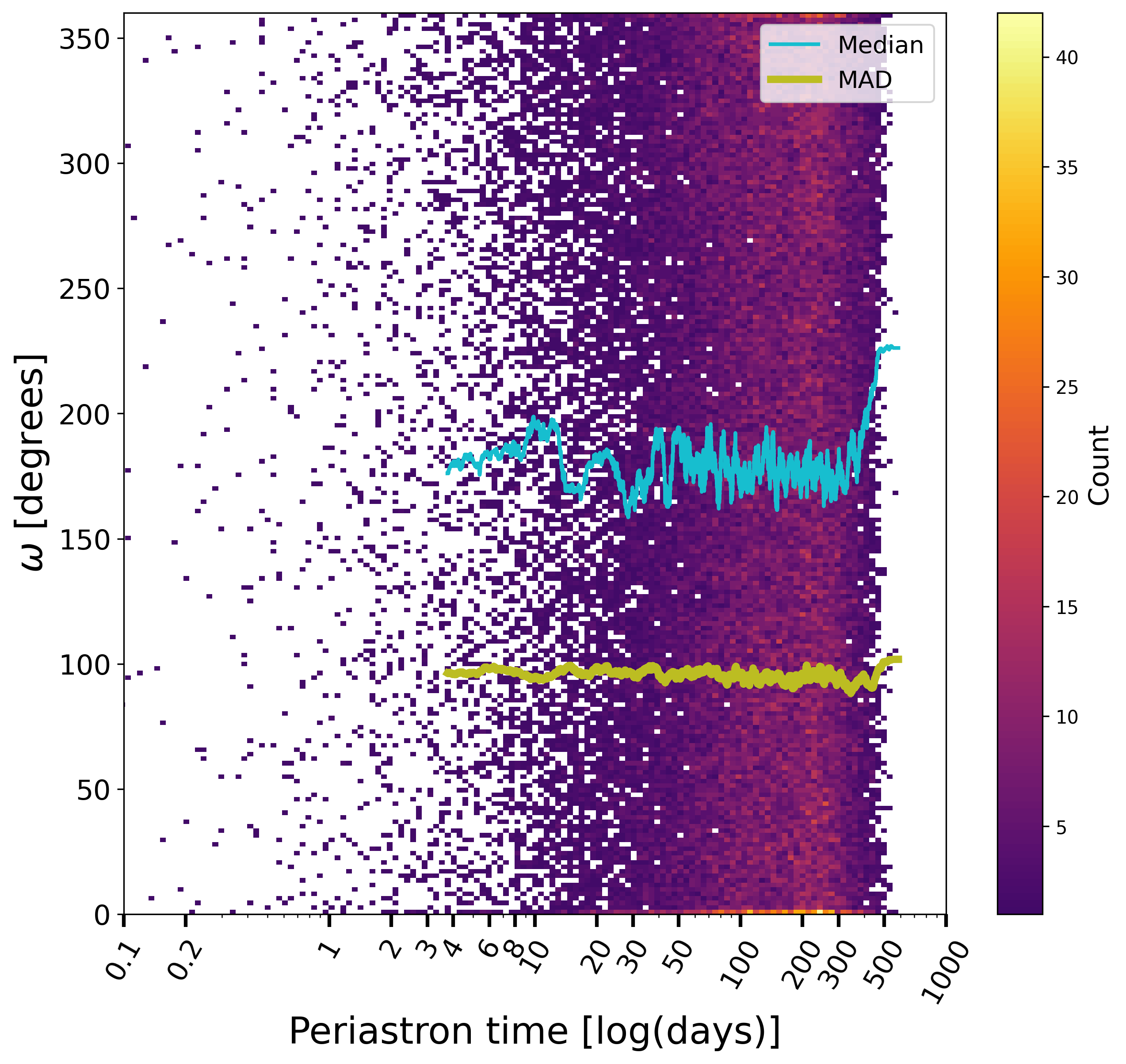
The statistical distributions for some of the estimated or derived parameters provide useful verifications of the processing which has been done. For example, the time of periastron over period, Figure 7.12, is reasonably uniform, except at the largest periods, where sources near periastron are more easily detected, as expected. This is also the case for the argument of periastron and cosine of the inclination where no special bias can be seen, beside the expected effect of low S/N solutions (Gaia Collaboration et al. 2023a).

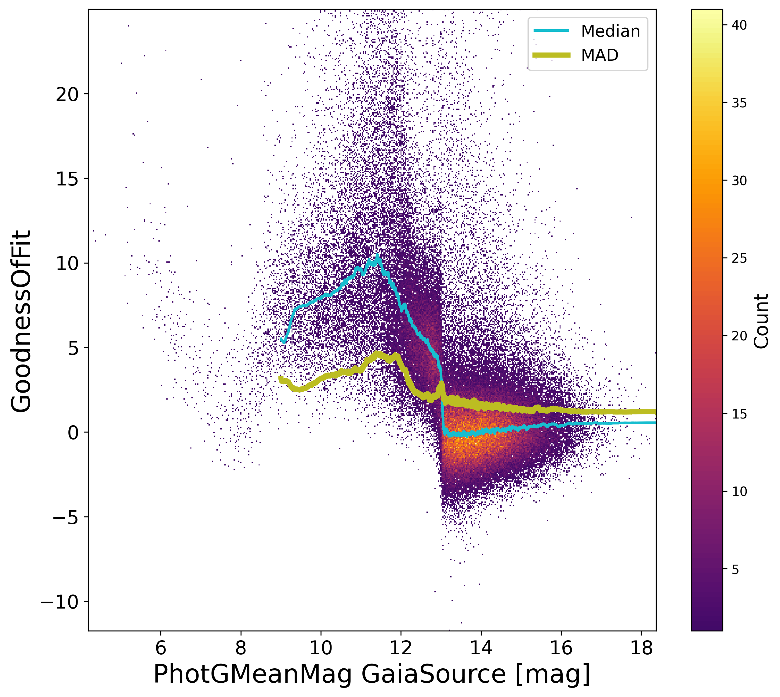
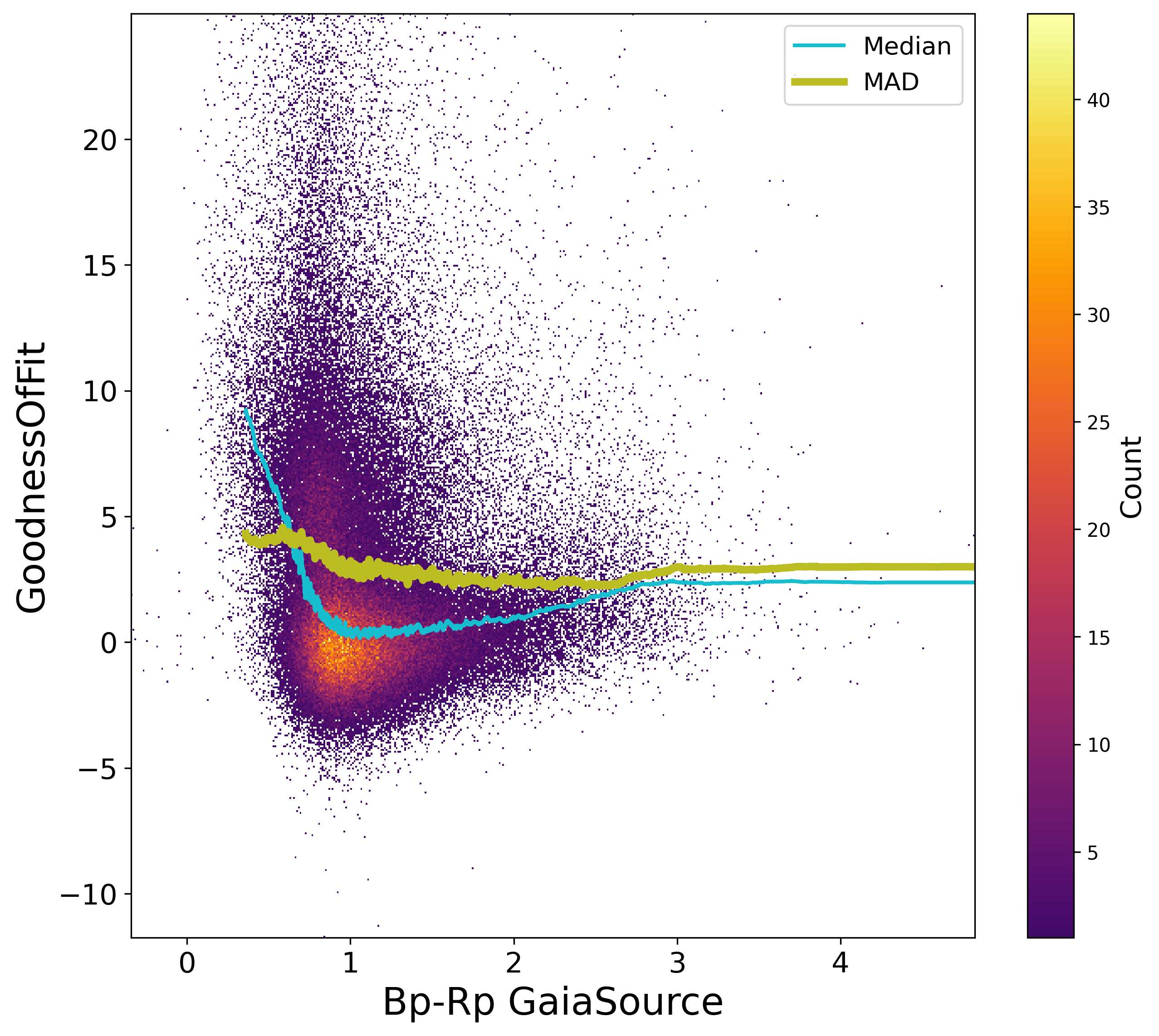
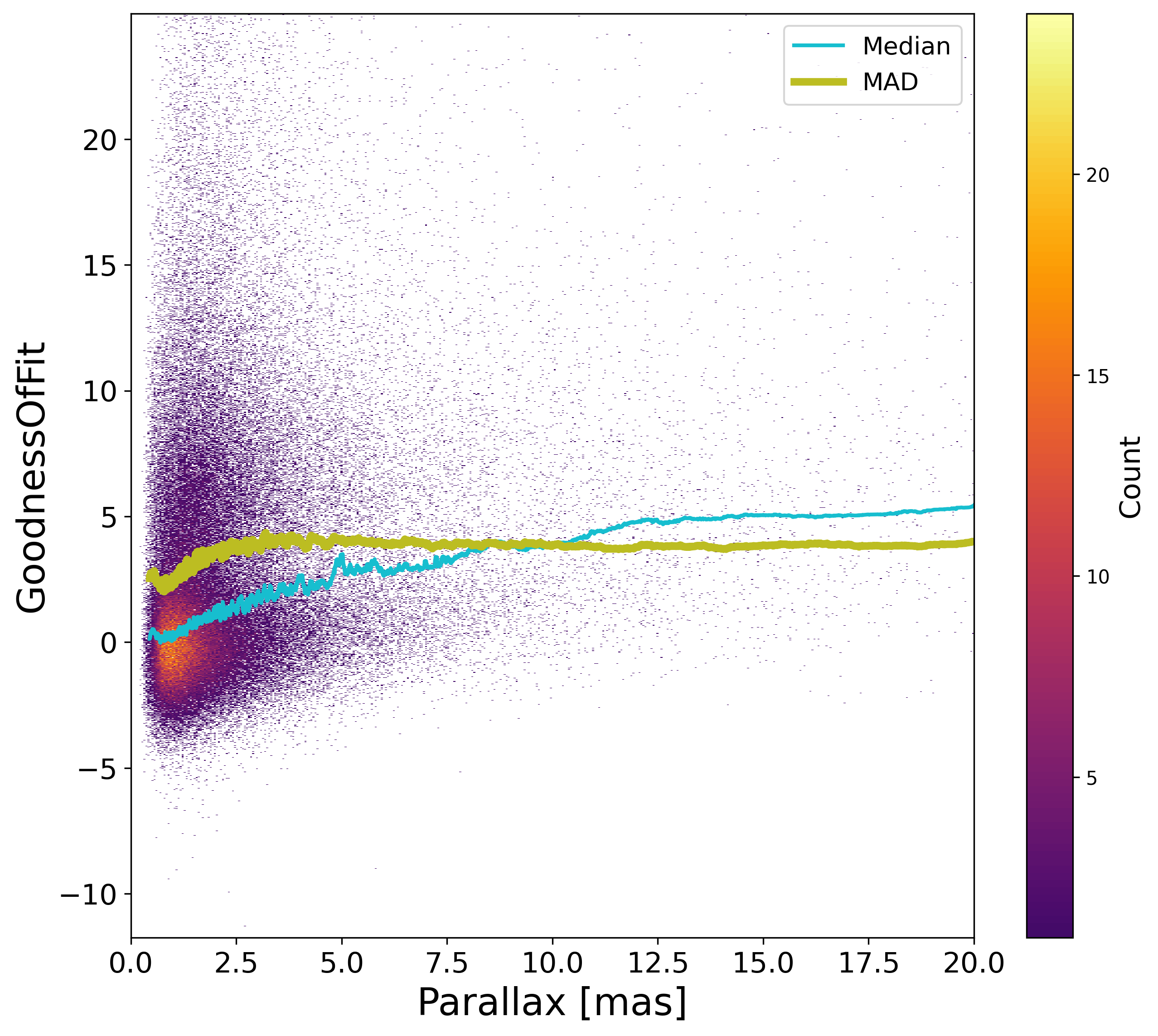
As judged using the goodness-of-fit, Figure 7.13, the quality of the solution however degrades for the bright sources, due to limitations of the calibration model, nearby sources, blue ones or giants. Fainter than $G>13$ and for more distant sources, the GoF is as expected around 0.

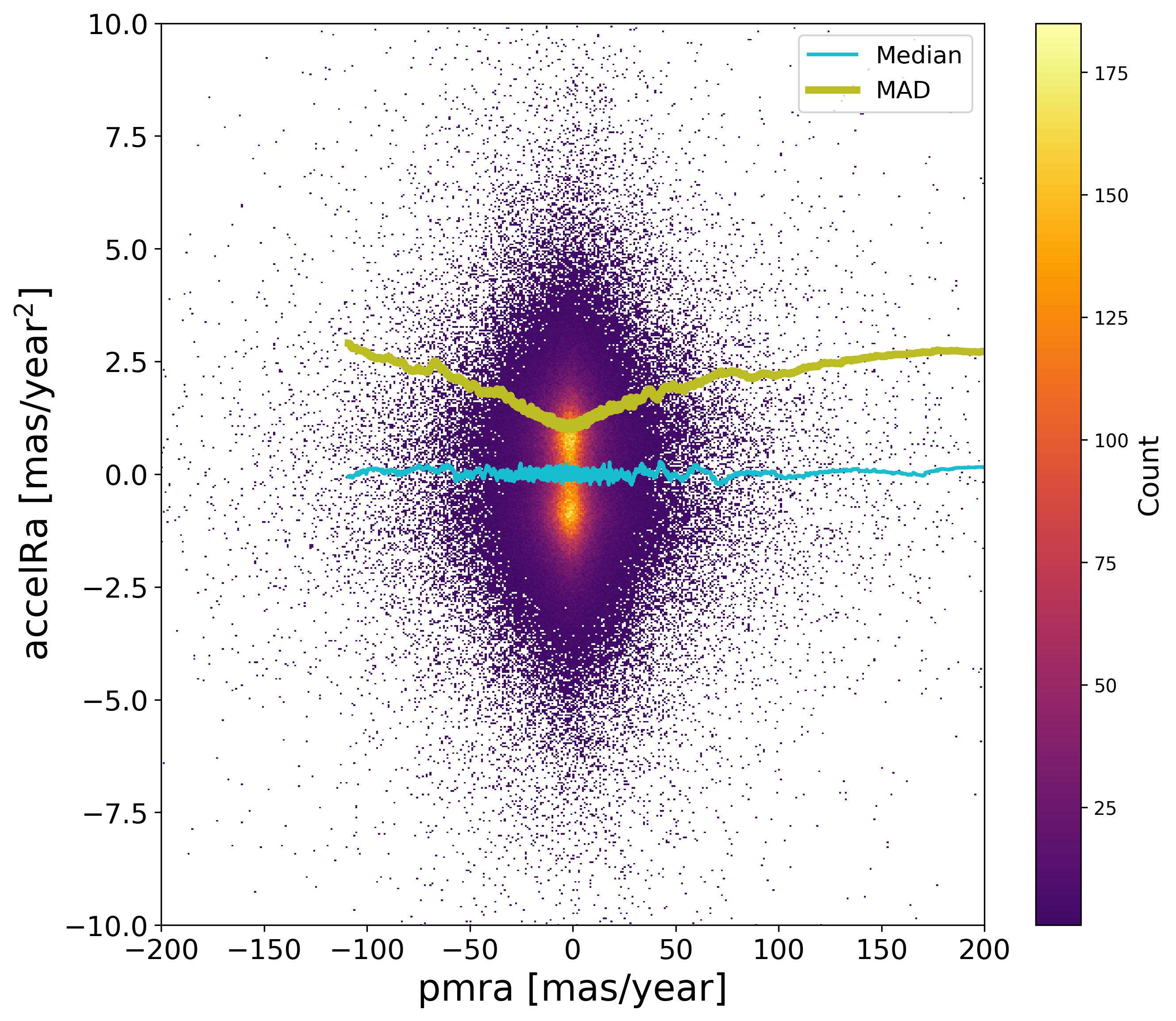
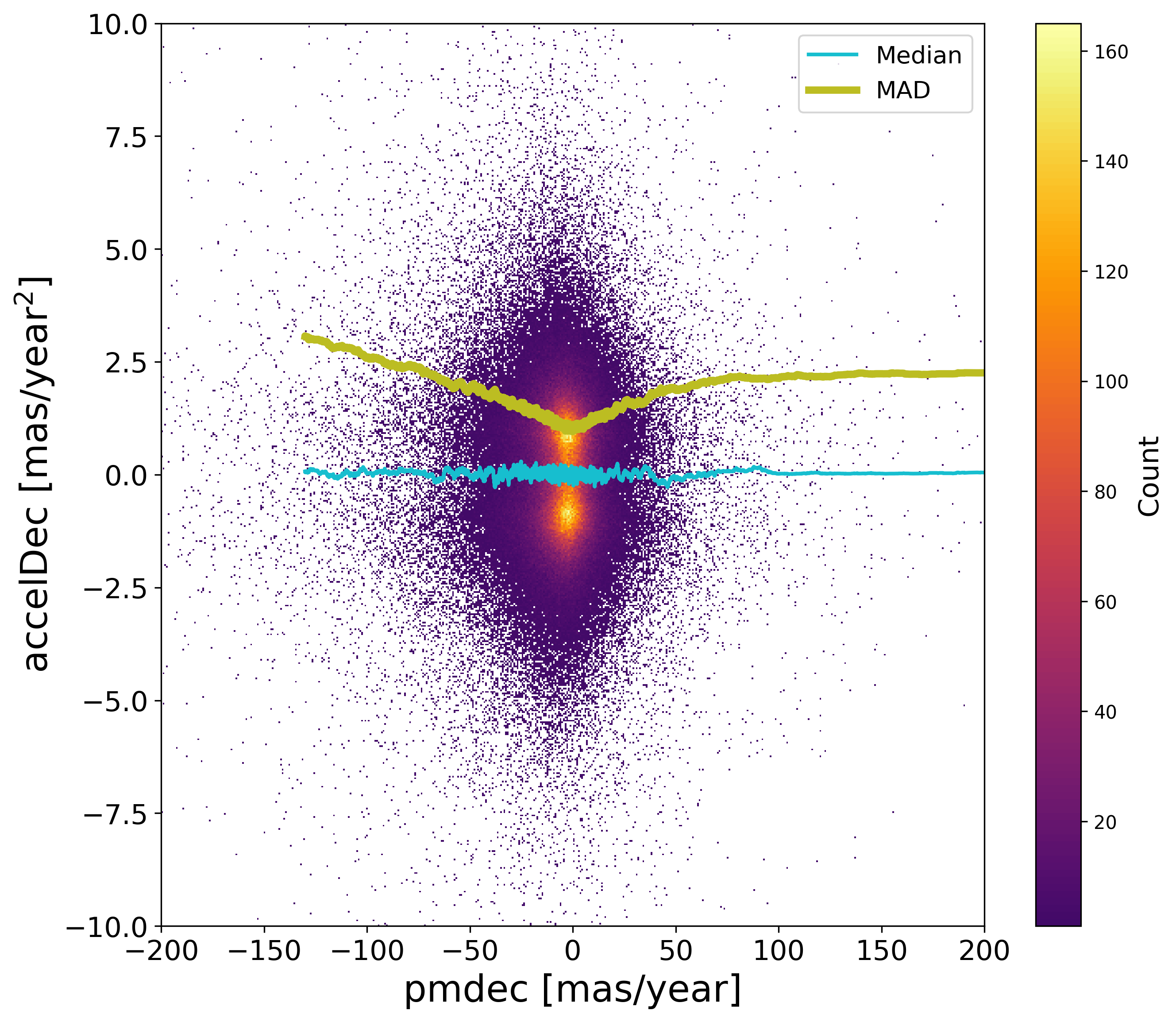
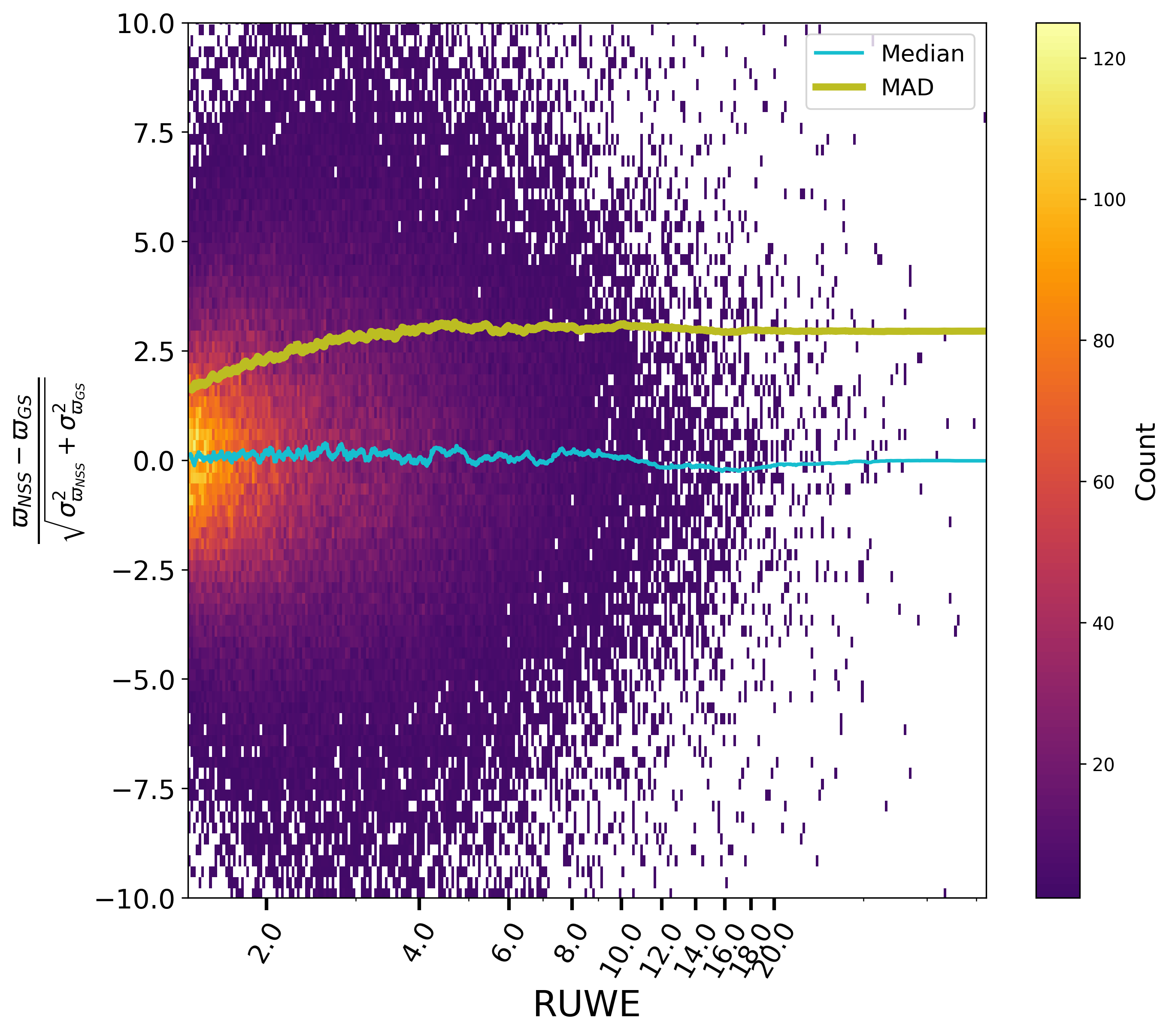
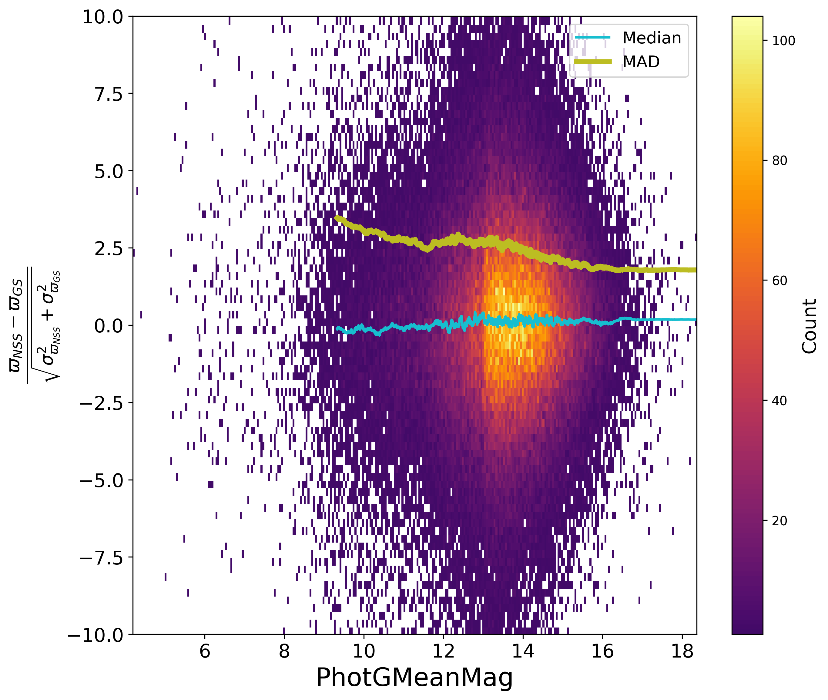
Concerning the acceleration solutions, the distribution of the acceleration components shows no apparent bias, Figure 7.14. Beside, one useful test is to check whether these solutions have indeed improved the astrometric solutions published for Gaia DR3 where sources had been managed as single stars. For this purpose, comparing the quality statistics such as the goodness-of-fit is not useful, due to the different handling of the solutions. Comparing the parallaxes is however possible, and Figure 7.15 suggests that there is no visible bias on the parallax. As for the estimation of the uncertainties however, these plots show firstly that either Gaia DR3 or the acceleration solutions have underestimated the formal uncertainties, as the normalised differences of these parallaxes, being correlated, should have a dispersion smaller than 1 while there are above 1.5. In principle, it is expected that the Gaia DR3 solutions are more robust, so it is unclear whether the increase of the MAD with ruwe may be due to an underestimation of the Gaia DR3 uncertainties or from a contamination from partially resolved double stars. It would not be unexpected that the larger dispersion for bright stars would be due to calibration issues not robustly being handled in the acceleration solutions, though.

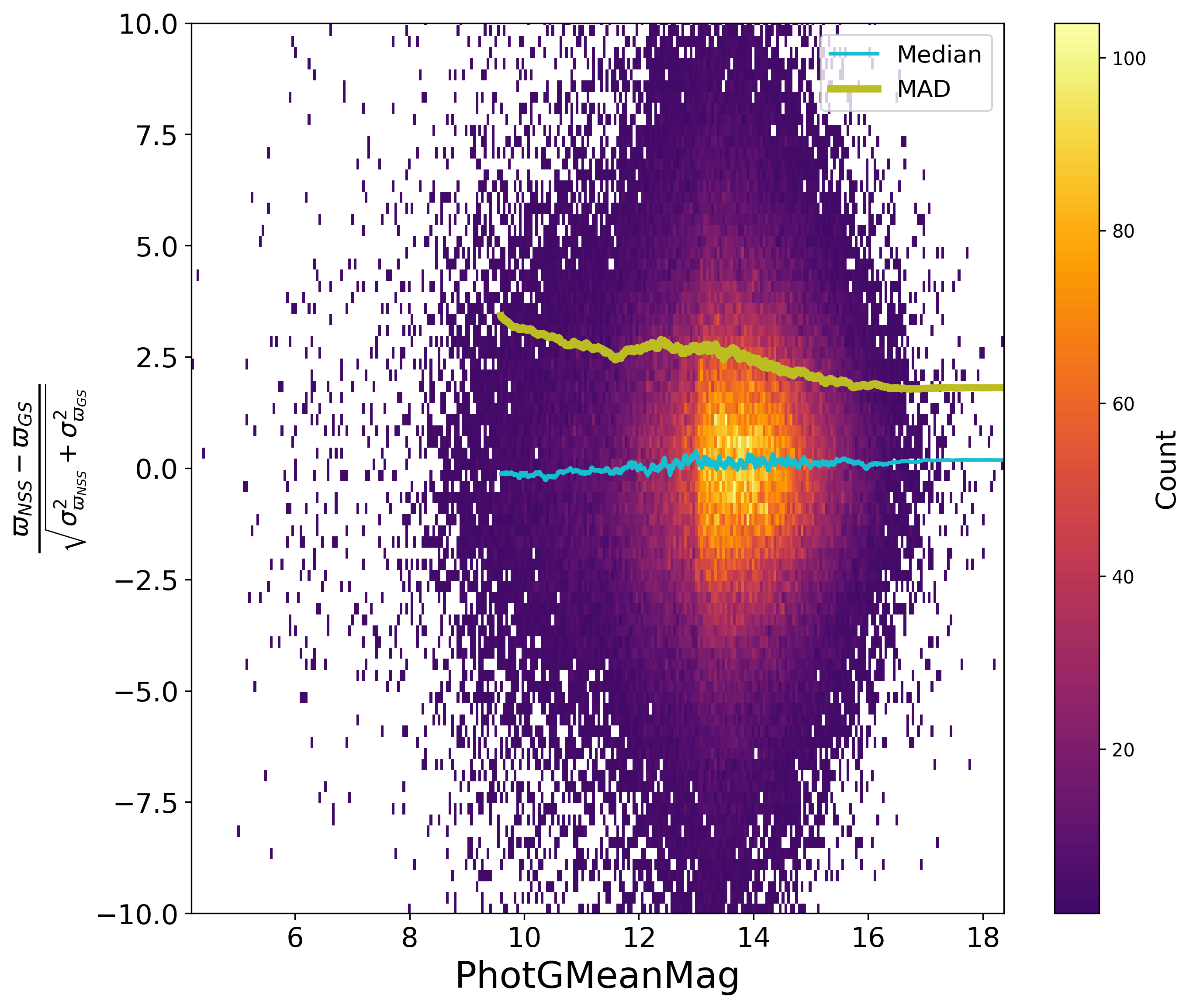
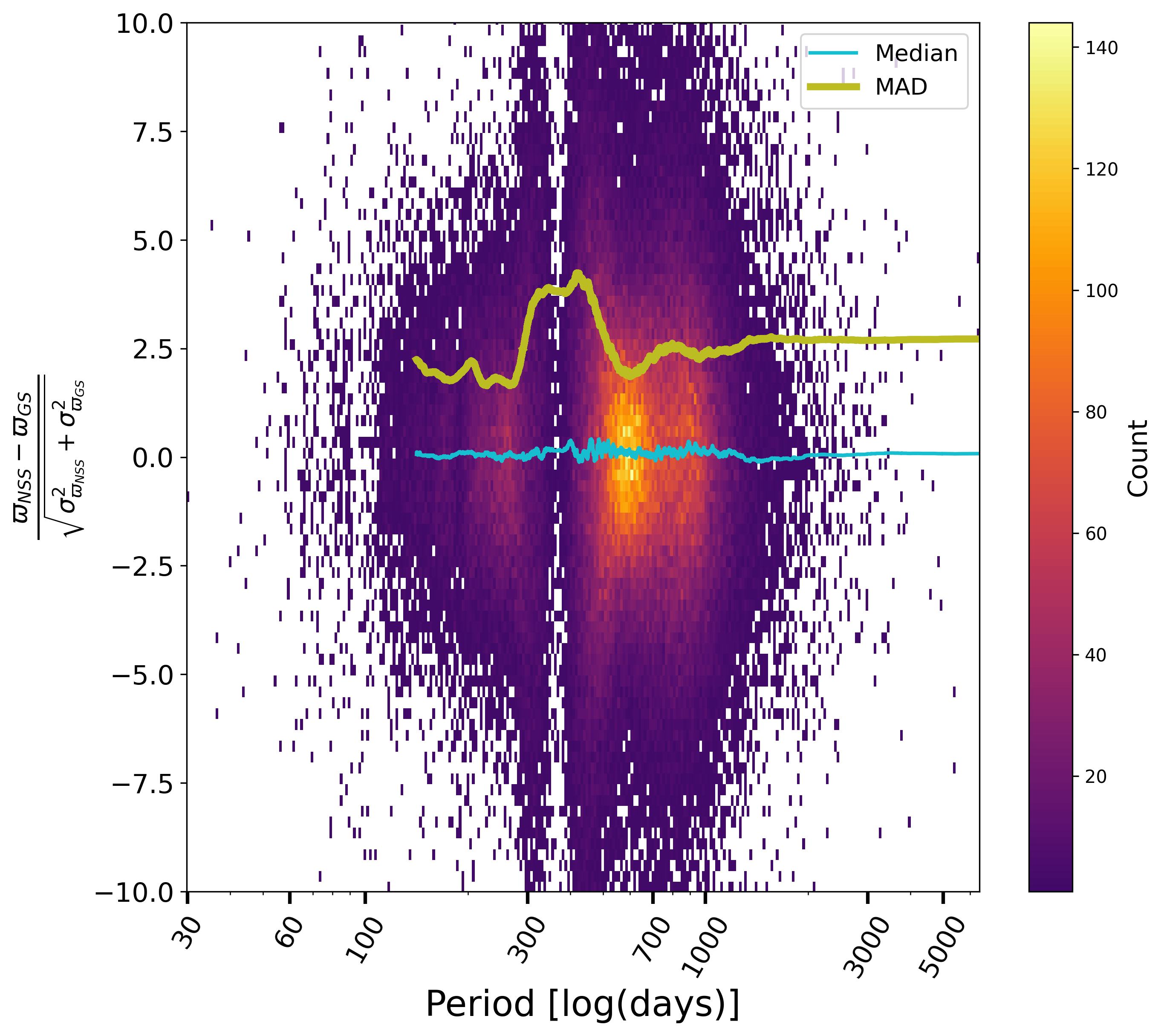
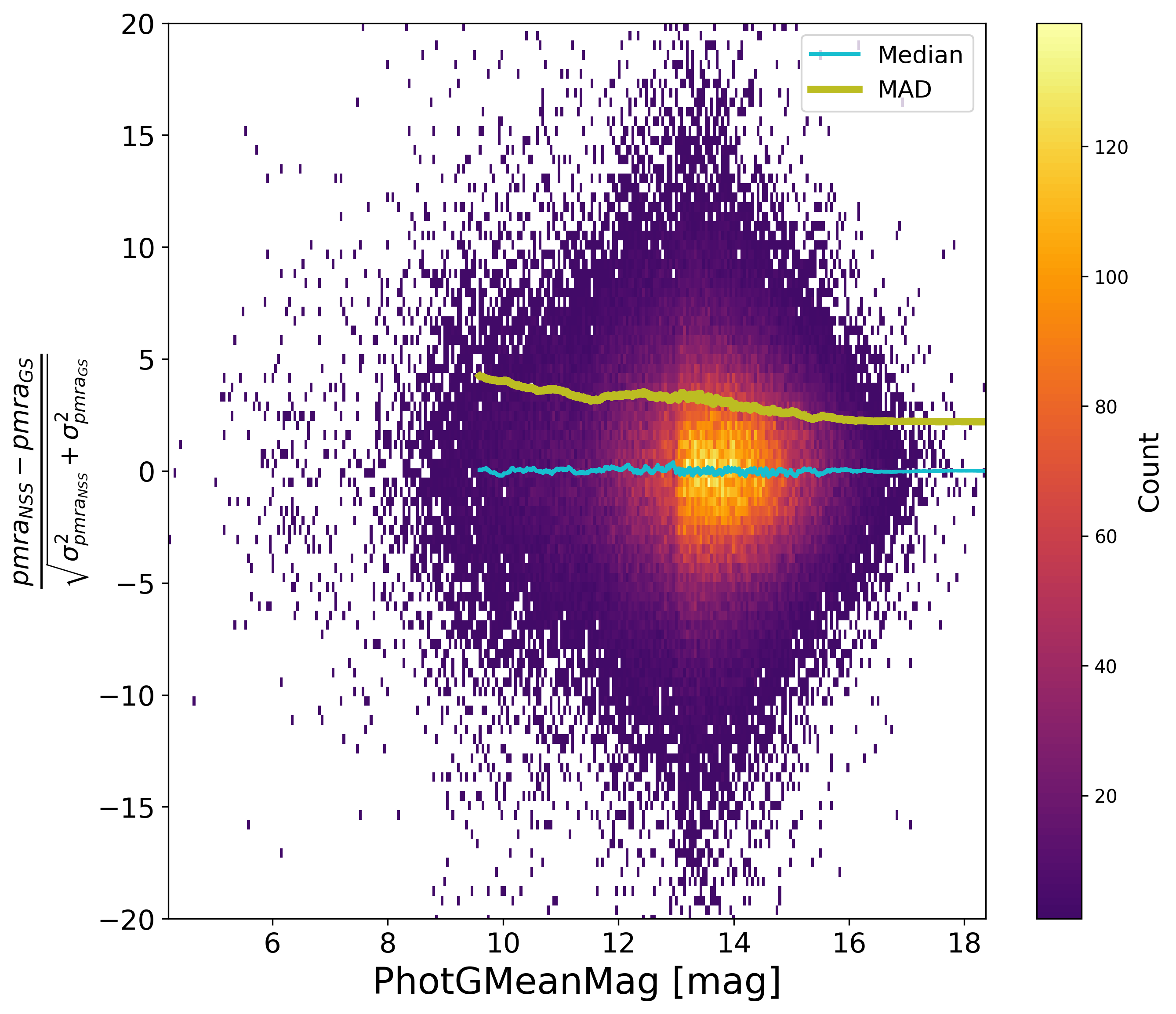
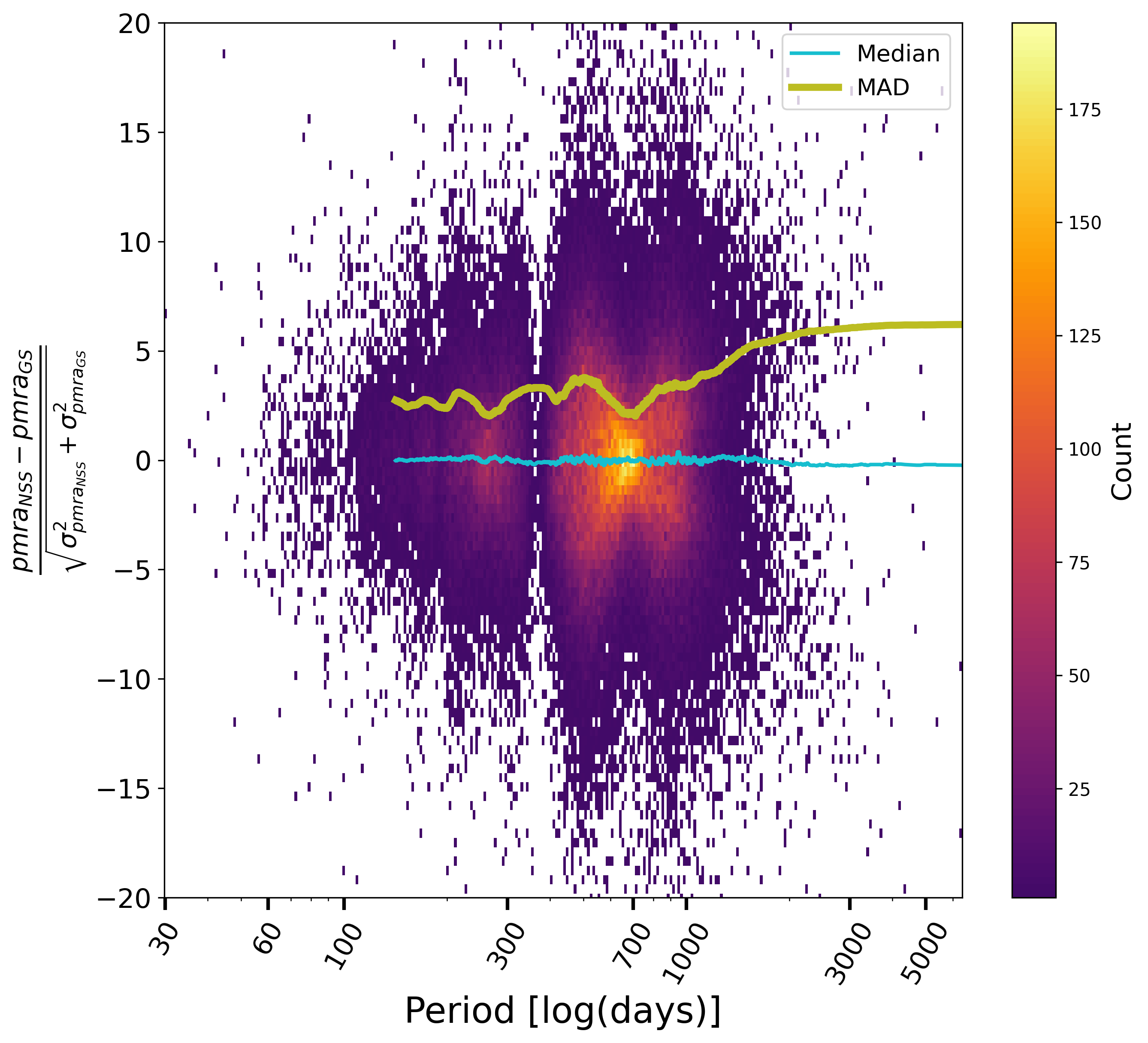
Comparing the parallaxes of orbital solutions to their value as estimated for Gaia DR3 with a single star model, Figure 7.16, is also instructive. No significant bias appears, but the dispersion on the parallax differences suggests that the Gaia DR3 parallaxes suffered for the brightest stars or periods around one year, and consequently that the NSS solutions significantly improved the astrometric parameters in this case. Figure 7.17 shows the normalised differences of the proper motions for orbital solutions compared to the Gaia DR3 ones. Again, there is no apparent bias, however it is well possible that the longer the period, the more the Gaia DR3 proper motions may have been contaminated, which appears statistically as a larger dispersion. Besides, for both parallax and proper motion, the formal uncertainties have been underestimated, without being able to attribute this to one or the other estimations, or to both.

Comparisons of the orbital parameters to external estimations have been done and are presented below, Section 7.7.4, with the 9th Catalogue of Spectroscopic Binary Orbits (Pourbaix et al. 2004, hereafter SB9) and the Sixth Catalog of Orbits of Visual Binary Stars (Hartkopf et al. 2001, hereafter Orb6) and this section concentrates here on alternative, complementary comparisons more statistically significant.

Thanks to the large number of NSS solutions, it indeed happened frequently that sources received both astrometric and spectroscopic orbital solutions. As the detection and processing of these two kind of orbits were done for completely different data in two completely different chains, the comparison represents a useful validation of both chains. One caveat is obviously that the two solutions should concern the same orbit, not the inner (for spectroscopy) plus the outer (for astrometry) orbits of a ternary system wrongly considered as binary only. For this purpose, only the systems with periods consistent within $5\times$ the uncertainty of the period difference were kept. A large fraction of these were subsequently combined (cf. Section 7.7) so what is presented in the following figures represents the initial astrometric and spectroscopic orbital solutions which have not been published, as they have been replaced by the combination of the two solutions.

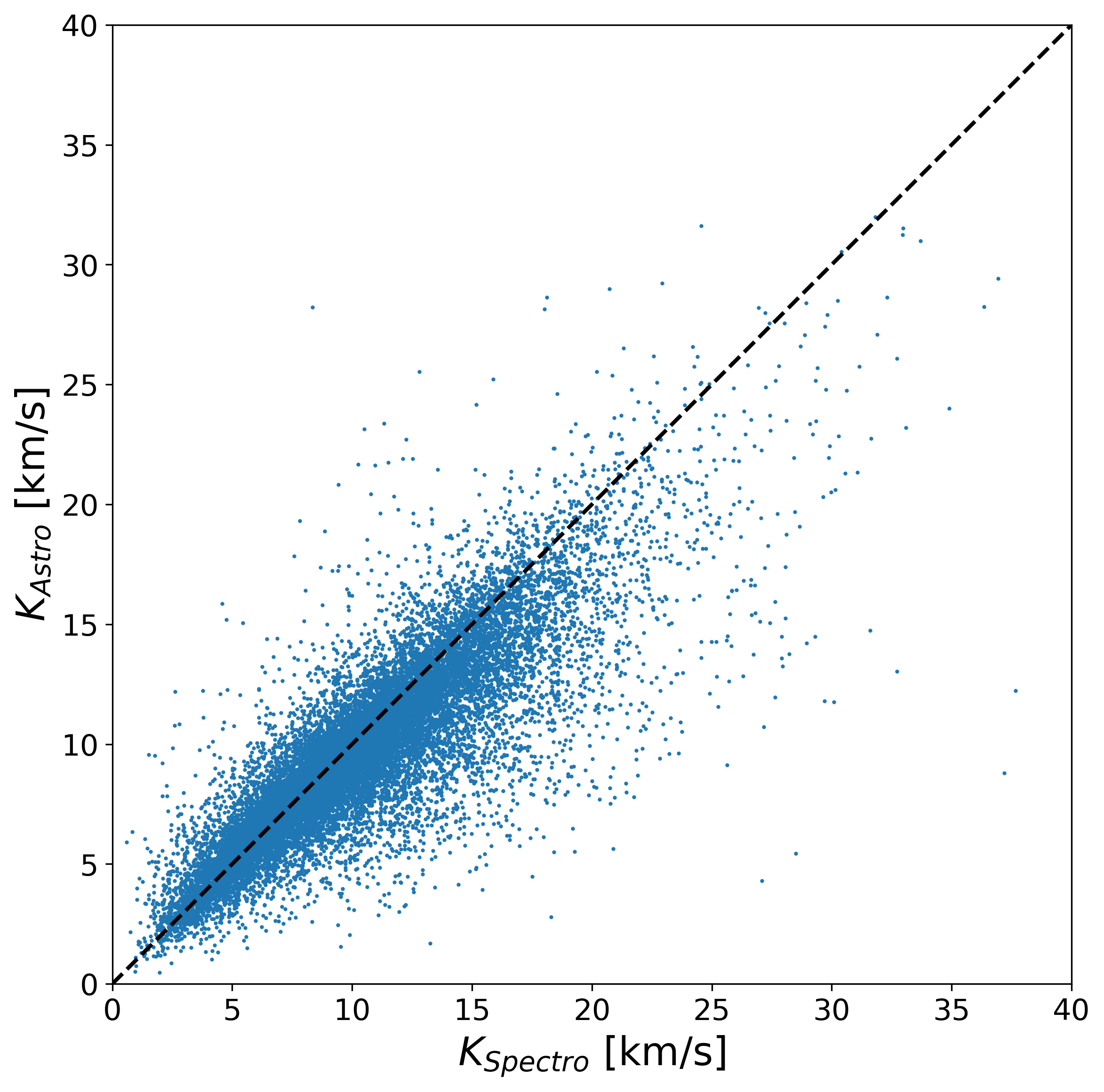
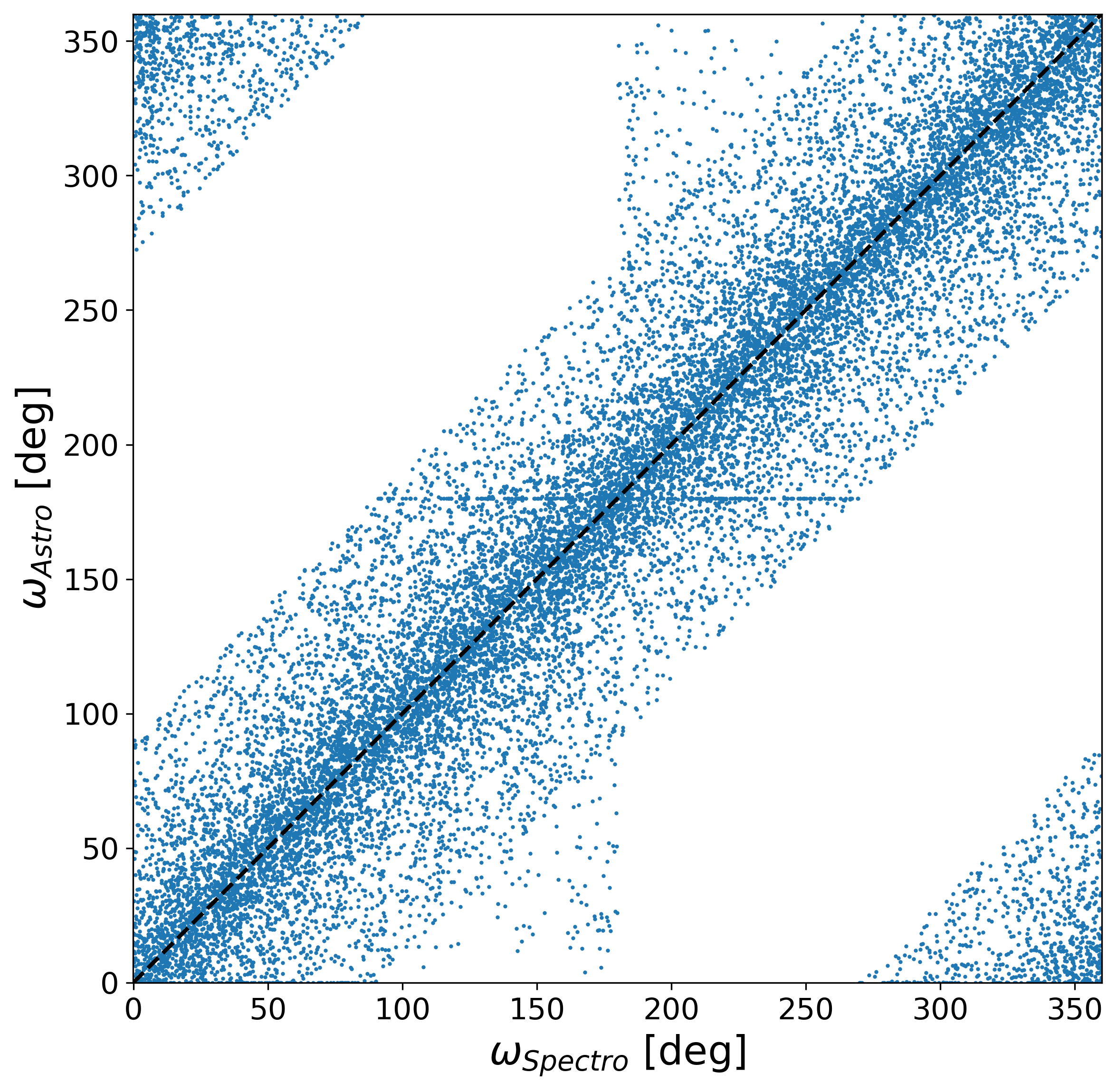
Converting the Thiele-Innes elements from the orbital astrometric solution into corresponding Campbell elements, one gets access to the semi-major axis of the photocentre $a_0$ and to the argument of periastron (e.g. Equation 7.15). Although a large dispersion is present for the latter, the comparison of astrometry to spectroscopy shows no apparent bias Figure 7.18b. One can also compute an “astrometric semi-amplitude” of the photocentre, i.e. substituting $a_0$ to $a_1$ in Equation 7.50 and compare it to the spectroscopic semi-amplitude. Figure 7.18a, the observed asymmetry is expected as $a_0\le a_1$ by definition, but the upper diagonal gives at least a hint of the uncertainties in play, below a few $\mathrm{km}{\mathrm{s}}^{-1}$ for most sources.

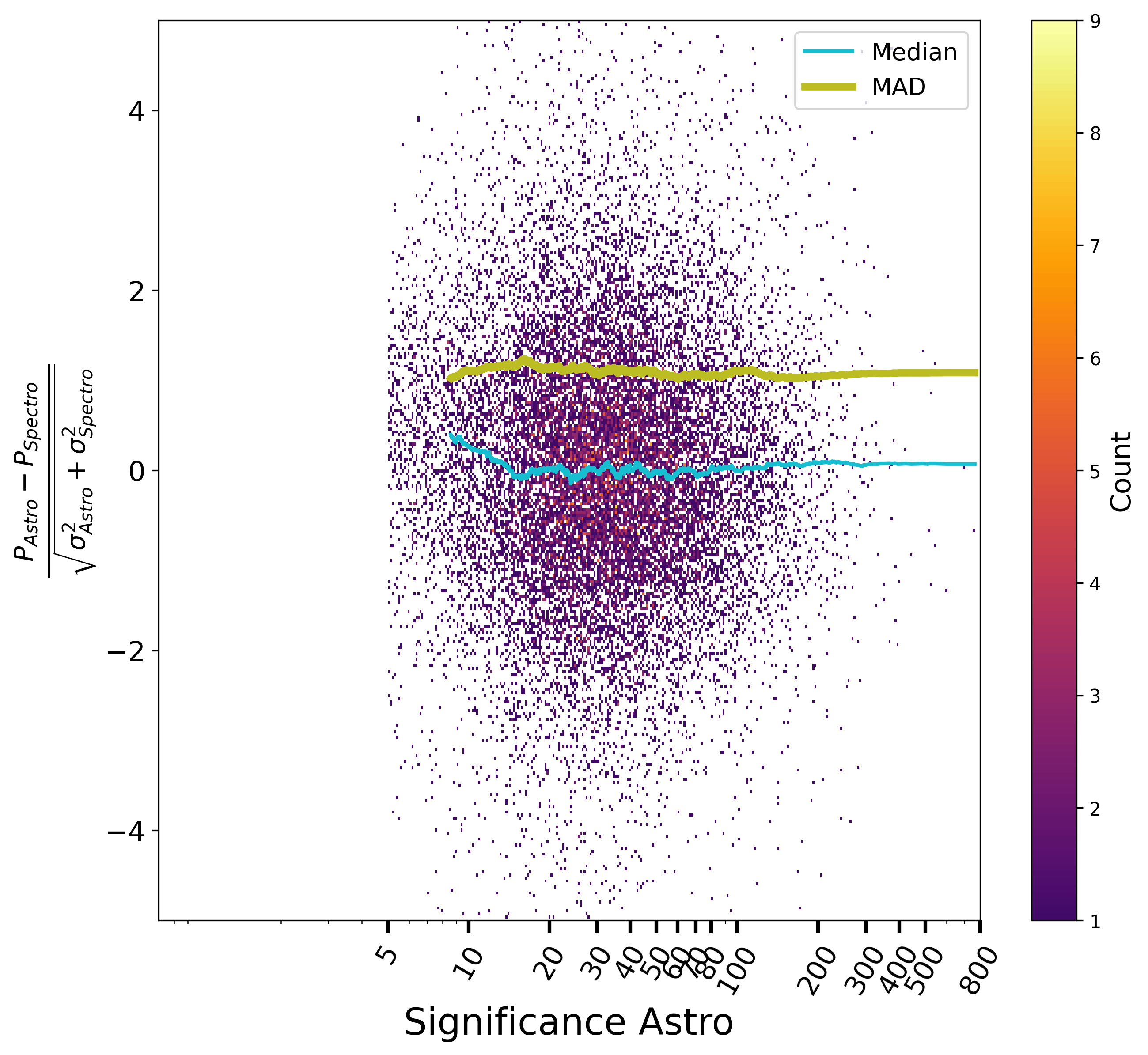
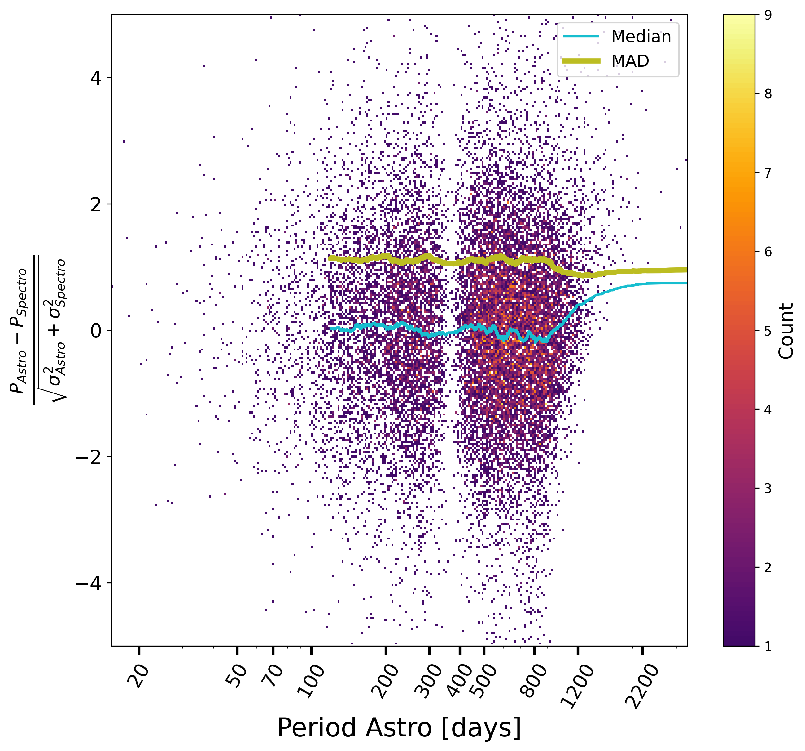
There is no apparent bias on the period, as judged from the normalised differences between astrometric and spectroscopic orbits, Figure 7.19a, except a slight one perhaps on the astrometric solution at low significance and small periods; on the contrary, the effect at large periods, Figure 7.19b, would rather be attributed first to the correlations of random errors between the ordinate and the abscissa, second to the spectroscopic part, which has less measurements and a lower sensibility. As for the uncertainties on period, they do not look too much underestimated.

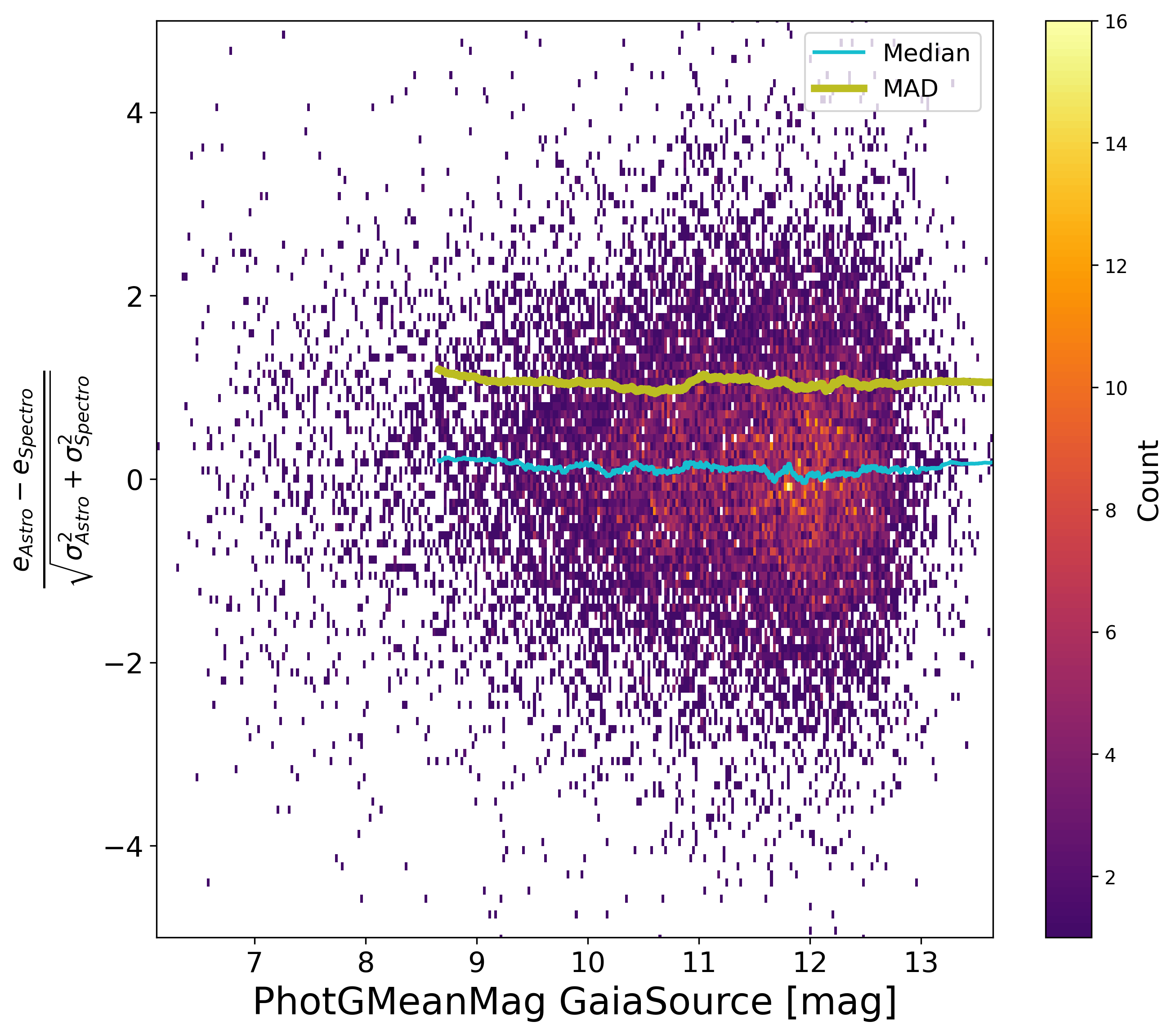
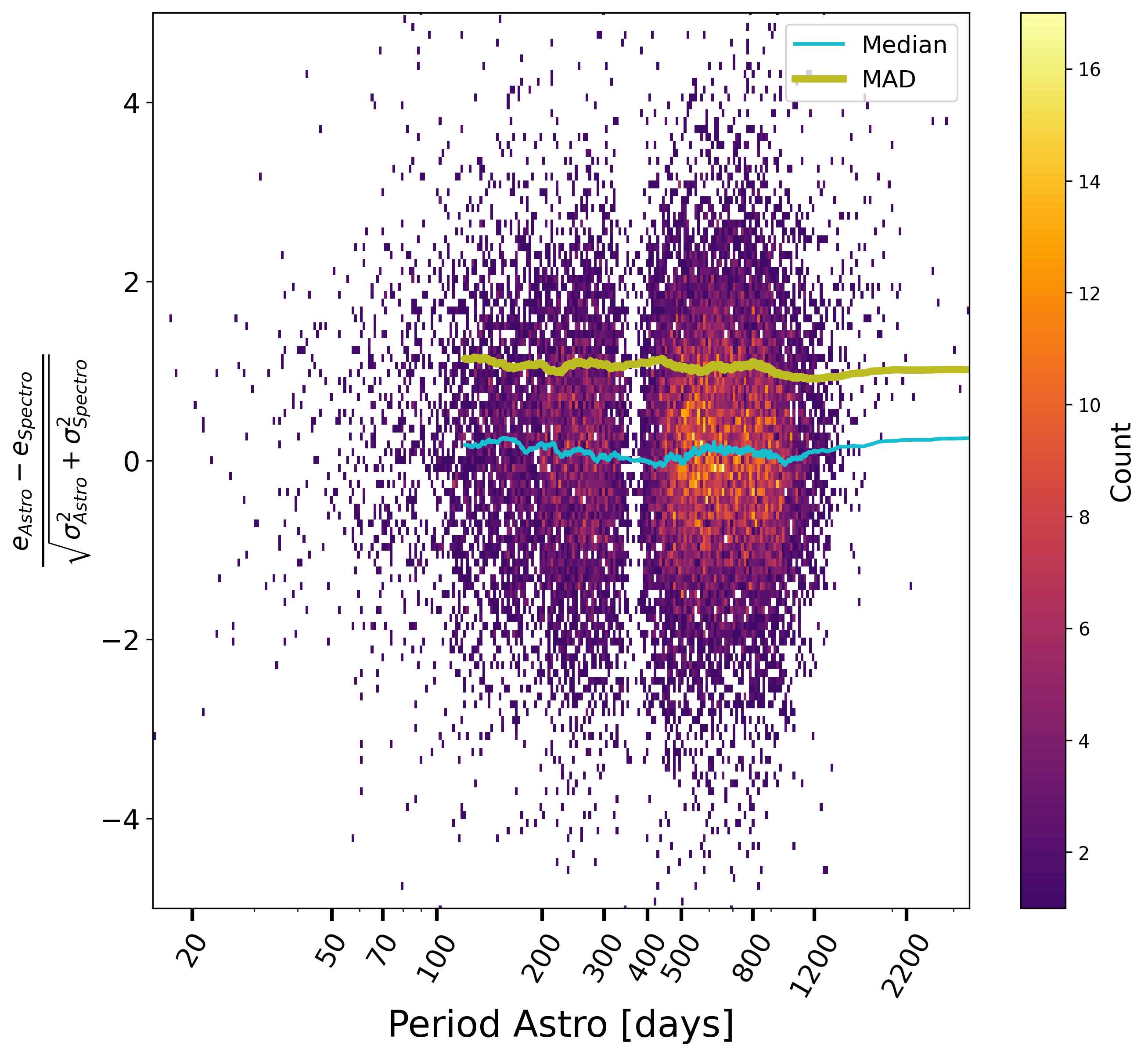
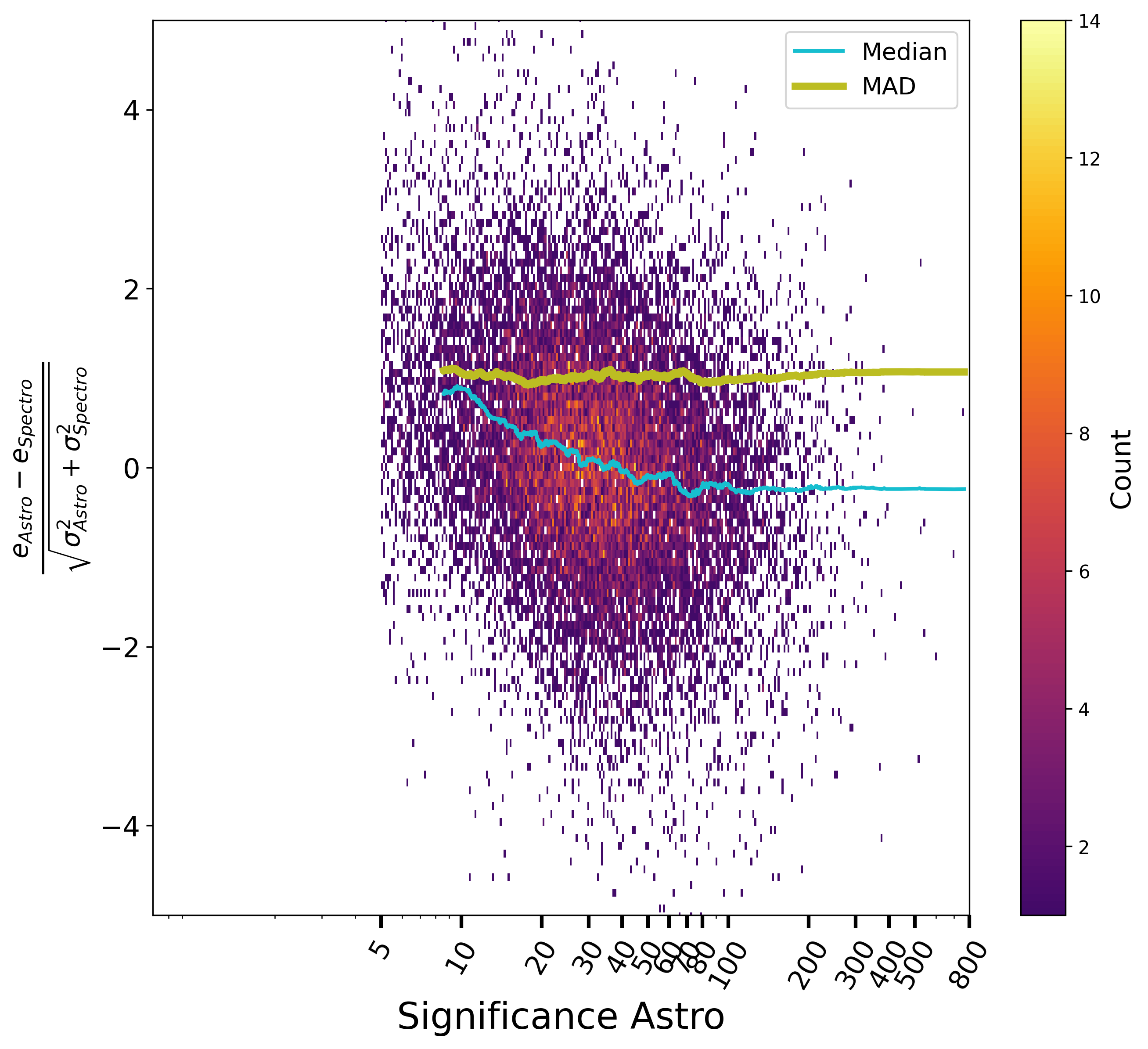
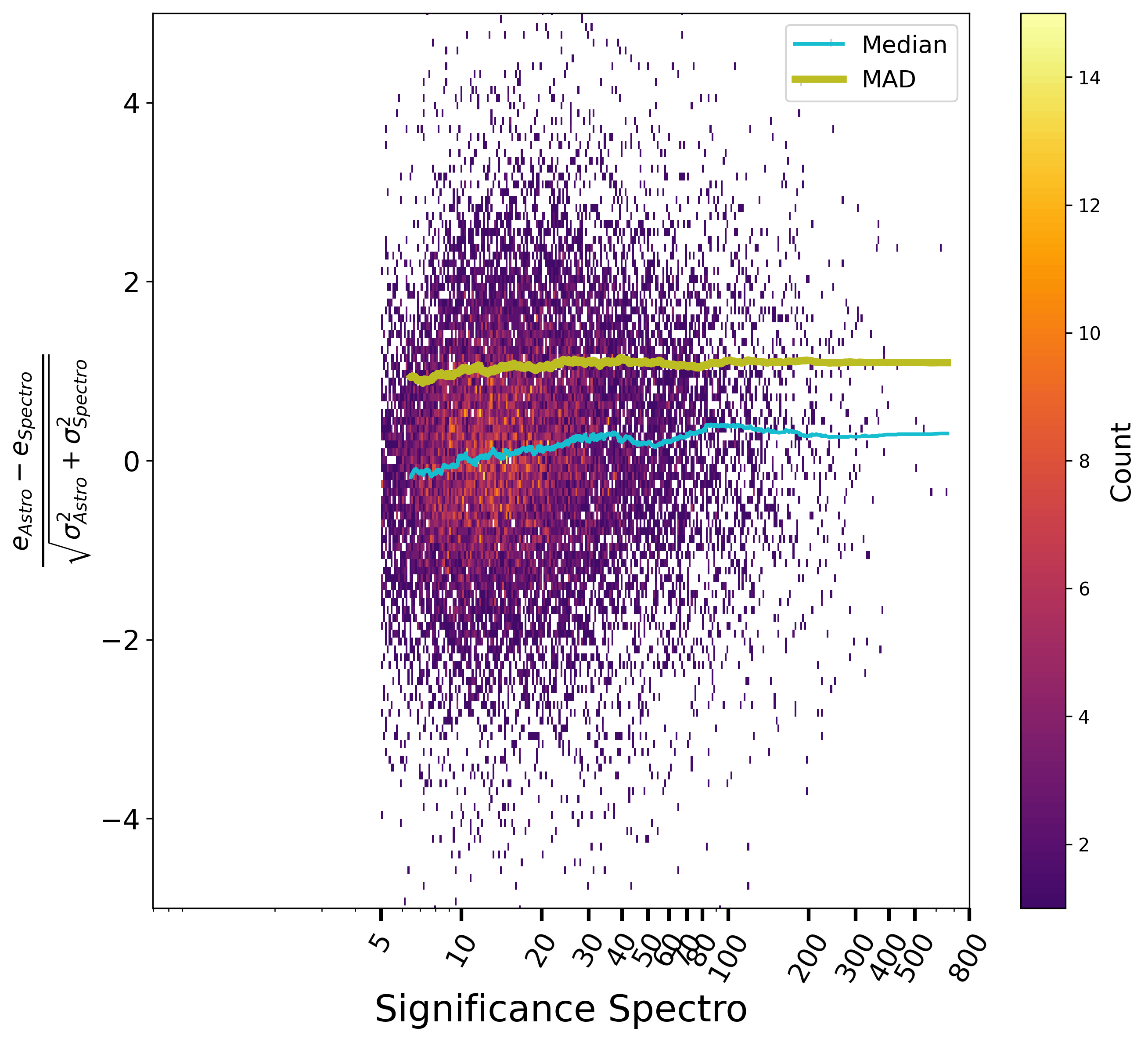
Concerning now the eccentricity, the normalised differences between astrometric and spectroscopic orbits vs. $G$ magnitude, period and significance of both solutions are shown respectively Figure 7.20 and Figure 7.21. There are no special systematics with magnitude or period, and no large underestimation of the formal uncertainties either. There is however as small bias on the eccentricity that is again attributed to the astrometric side as it is decreasing when the astrometric solutions becomes more significant, while not present at low S/N spectroscopic orbits. The level of the systematic effect stays however below the random error.