7.2.5 Orbital solutions
Calculation of orbital solutions
The orbit of a binary system is generally described by seven parameters: the first three are the period, , the epoch of periastron passage, , and the eccentricity, . Then come the semi-major axis of the orbit described by the photocentre, , the inclination of the orbital plane with respect to the sky, , the position angle of the ascending node, , and the periastron longitude measured from the ascending node, . The precise definition of these parameters can be found in any astronomical handbook dealing with double stars (see, e.g. Binnendijk 1960; Heintz 1978). These four parameters are called Campbell’s elements, and each measurement of the position of the photocentre relative to the barycentre of the system is related to these elements by a completely non-linear relationship.
The calculation of the orbital solutions is made partly linear by replacing the Campbell elements by the Thiele-Innes elements. These, denoted by the letters , , and , are related to the Campbell elements by the following relations:
| (7.12) |
and the along-scan abscissa of the photocentre is then given by the equation:
| (7.13) |
where , and are the same as is Section 7.2.4; is the eccentric anomaly, which depends on the epoch by the relation:
| (7.14) |
As depends on five unknowns, the orbital solution finally has twelve unknowns, nine of which enter into a linear relationship. The solution is therefore sought by exploring the space defined by , and with the Levenberg-Marquardt method. For each star, the period interval at the beginning of the calculation goes from 10 days to the duration covered by the observations divided by 0.6.
Significance of orbital solutions
The significance of the orbital solutions is defined as , since a semi-major axis as small as its uncertainty corresponds to an orbit that may well not exist. However, and its uncertainty must be deduced from a solution that has been calculated in Thiele-Innes elements. For that purpose, the formulae provided by Binnendijk (1960) has been used:
| (7.15) |
The uncertainties of the Campbell’s elements may be derived from , , , and from the variance–covariance matrix (Halbwachs et al. 2023); for the semi-major axis, one obtains:
| (7.16) |
where is the term of the variance–covariance matrix corresponding to the (, ) pair, ie . The significance of the orbital solution is then estimated.
From small eccentricity orbits to pseudo-circular orbits
Orbits with small eccentricities are a problem because the uncertainties of the Thiele-Innes elements are much larger than the elements themselves. In addition, the uncertainty on can greatly exceed the value of the period. These defects come in fact from the indeterminacy of the periastron, which affects , but also . However, if the uncertainties of the Campbell elements are derived from the solution obtained with Thiele-Innes elements, one may note that the problem is primarily one of presentation, since , and actually have very acceptable uncertainties. Nevertheless, it was decided to transform the orbits with eccentricity , not by circularising them, but only by fixing the eccentricity and by shifting the periastron to the ascending node (obviously, such an operation is only possible because the uncertainty of the eccentricity is always much greater than 0.0005). Orbits transformed in this way are called pseudo-circular orbits hereafter. This transformation was achieved with several steps:
-
•
The Campbell elements were derived from the Thiele-Innes elements, and the Thiele-Innes elements were computed again, assuming in Equation 7.12.
-
•
After this operation, it is easy to see that and . Therefore, only 3 of the 4 Thiele-Innes elements are considered as unknowns. has been arbitrarily discarded, checking first that is always larger than ; otherwise, would have been chosen instead of .
-
•
The periastron epoch has been shifted by subtracting the time so as to correspond to the passage at the ascending node.
-
•
The variance-covariance matrix has been recalculated for the remaining ten unknowns, since was discarded and is considered as fixed to its initial value.
-
•
The resulting matrix is transcribed into a matrix, with the terms corresponding to the discarded unknowns set to zero.
It should be noted that, in reality, the uncertainties and correlations of and are not zero nor NaN, although they appear so in the delivered solution. It is up to the users to identify the solutions treated in this way (identified by the condition eccentricity_error is NaN), and to use them appropriately. For example, the uncertainty on , (resp. , ) may be estimated from the propagation of the uncertainties of the three other elements, thanks to the equation:
| (7.17) |
A user wishing to calculate the uncertainties of the Campbell elements using the equations of Halbwachs et al. (2023) will still need the correlation coefficients relating to the other Thiele-Innes elements. Since , one has:
| (7.18) |
These recommendations also apply to the few calculated circular orbits (there are only 8 at the end of the calculation), which are presented in the same way.
Initial selection of orbital solutions
As with the acceleration solutions, a dynamic criterion was used to ensure the plausibility of the solution. We considered the astrometric mass function, defined as:
| (7.19) |
where is derived from Equation 7.15, is in the same unit as and is the period in days to have in solar masses, . Since corresponds to the orbit of the photocentre, is a function of the masses of the components, and , and also their fluxes, and , as shown in the equation:
| (7.20) |
Since the more massive component is usually much brighter than the other, the index “1” is assigned to the brightest component, and is neglected. The maximum value of is then:
| (7.21) |
where is the mass ratio. The largest possible value for , obtained when is then . This limit has been adopted, keeping in mind that it is a bit optimistic since components of the same mass should have identical fluxes, and therefore a zero semi-major axis.
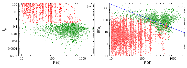
Some of the orbital solutions derived in a trial processing are shown in Figure 7.6. It can be seen that the reliable solutions have a mass function of less than 0.3, and that, as expected, periods close to one-year are almost absent. For their part, the doubtful orbits populate very specific periods, such as 1 year, 6 months, or harmonics of the year and the precession period of the satellite (63 days), cf. Holl et al. (2023a).
Figure 7.6(b) shows the same solutions in the period vs. “significance of the parallax” (i.e. ) diagram. It can be seen that the dubious solutions, in red, encroach on the domain of valid solutions, but that it is nevertheless possible to avoid them with the condition:
| (7.22) |
Such a selection means in fact accepting short-period solutions only when they concern nearby stars. It has the advantage of effectively eliminating doubtful solutions (including those with small mass functions, but which are identifiable by their concentration on particular periods) without radically preventing the detection of binaries with a truly large mass function. For these reasons, it has been included among the acceptance criteria considered during processing, along with the basic criteria presented in Section 7.2.3.
Final selection of the orbital solutions
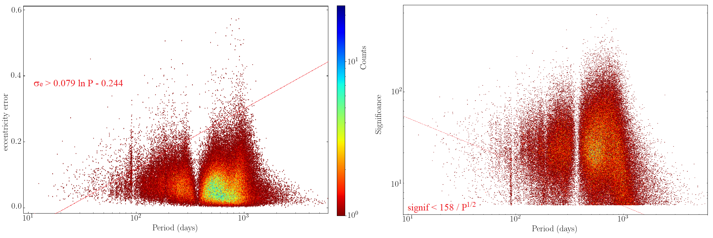
After processing, the alternative solutions that had been accepted with were rejected, because the proportion of mass functions greater than 0.3 was significantly higher than the value found for : 1.75 % instead of 1.05 %. After that, the rate of large mass functions could hardly be improved, but there remained many solutions concentrated around specific periods. Considering the diagrams linking the period to the other parameters, it appeared from Figure 7.7 that the following two selection conditions avoid most of these doubtful orbits. These are:
| (7.23) |
and a filter based on the significance:
| (7.24) |
After this last filtering, 166 500 astrometric orbits were retained, including about 1% of mass function exceeding 0.3.