7.2 Astrometric binaries 7.2.3 Acceptance of solutions 7.2.5 Orbital solutions

7.2.4 Acceleration solutions

Calculation of acceleration solutions

The acceleration models are the constant-acceleration model, which has 7 parameters, and the variable-acceleration model, which has 9 parameters. These models assume that the along-scan abscissa may be written as:

\begin{array}[]{rl}w=w_{\mathrm{ss}}&+\;\frac{1}{2}\left[t^{2}-\frac{\Delta T^% {2}}{3}\right]\times\left(\frac{\partial w}{\partial a}g_{\alpha*}+\frac{% \partial w}{\partial d}g_{\delta}\right)\\ &\\ &\left\{\;+\;\frac{1}{6}\left[t^{2}-\Delta T^{2}\right]t\times\left(\frac{% \partial w}{\partial a}\dot{g}_{\alpha*}+\frac{\partial w}{\partial d}\dot{g}_% {\delta}\right)\;\right\}\end{array}

(7.5)

were $w_{\mathrm{ss}}$ is the contribution of the 5-parameter single-star model, $\frac{\partial w}{\partial a}$ is the partial derivative of $w$ with respect to the local right ascension coordinate, $a$ , and $\frac{\partial w}{\partial d}$ is the partial derivative $w$ with respect to the local declination coordinate, $d$ , these two quantities being part of the single-star model (the astrometric models all give the position of the photocentre in the local plane coordinates, whose origin is a fixed point near the star). $g_{\alpha*}$ and $g_{\delta}$ are the equatorial coordinates of the acceleration, while $\dot{g}_{\alpha*}$ and $\dot{g}_{\delta}$ are their derivatives with respect of time. Therefore, the first line of Equation 7.5 is for the constant-acceleration model, while the last term between the braces should be added to obtain the variable-acceleration model. $t$ is the epoch measured from the reference epoch 2016.0. The term $\Delta T$ has been introduced so that the calculated position corresponds to the average position of the star, and not to a point on its trajectory. Similarly, the proper motion calculated by applying the 9-parameter model corresponds to the mean proper motion. In doing so, we are simply repeating the method used in the preparation of the Hipparcos catalogue (ESA 1997, volume 1, Section 2.3.3). In principle, $\Delta T$ is half the duration covered by the observations of each star. In practice, $\Delta T=517.5$ days was assumed, which is a little longer than the real value, but the difference should not have any consequence.

Initial selection of acceleration solutions

We must first define the significance before using it to make a selection. As in Hipparcos, the significance of the constant-acceleration model, $s_{7}$ , is the norm of the acceleration vector, divided by its uncertainty. It is derived from the equation:

s_{7}=\frac{1}{\sigma_{g_{\alpha*}}\sigma_{g_{\delta}}}\sqrt{\frac{g_{\alpha*}% ^{2}\sigma_{g_{\delta}}^{2}+g_{\delta}^{2}\sigma_{g_{\alpha*}}^{2}-2g_{\alpha*% }g_{\delta}\rho_{g_{\alpha*}g_{\delta}}\sigma_{g_{\alpha*}}\sigma_{g_{\delta}}% }{1-\rho^{2}_{g_{\alpha*}g_{\delta}}}}

(7.6)

where $\sigma_{p}$ refers to the uncertainty of the parameter “ $p$ ”, and $\rho_{g_{\alpha*}g_{\delta}}$ is the coefficient correlation between $g_{\alpha*}$ and $g_{\delta}$ .

The significance of the variable-acceleration model, $s_{9}$ , is defined in the same way, but on the basis of the derivative of the acceleration with respect to time. It is:

s_{9}=\frac{1}{\sigma_{\dot{g}_{\alpha*}}\sigma_{\dot{g}_{\delta}}}\sqrt{\frac% {\dot{g}_{\alpha*}^{2}\sigma_{\dot{g}_{\delta}}^{2}+\dot{g}_{\delta}^{2}\sigma% _{\dot{g}_{\alpha*}}^{2}-2\dot{g}_{\alpha*}\dot{g}_{\delta}\rho_{\dot{g}_{% \alpha*}\dot{g}_{\delta}}\sigma_{\dot{g}_{\alpha*}}\sigma_{\dot{g}_{\delta}}}{% 1-\rho^{2}_{\dot{g}_{\alpha*}\dot{g}_{\delta}}}}

(7.7)

Figure 7.4: Schematic diagram of the acceptance process of the acceleration solutions. The 9-parameter solution coming from the variable-acceleration model is considered before the 7-parameter solution, in order to accept the most complete solution, when it is relevant. $\Phi_{7}$ and $\Phi_{9}$ are the filter given in Equation 7.10 and Equation 7.11, respectively.

In order to check the plausibility of the solutions, constraints on the mass of the binary components were considered which are deduced from the acceleration of the photocentre. The acceleration projected on the sky, $\Gamma$ , was calculated first, with the formula:

\Gamma=\frac{\sqrt{g_{\alpha*}^{2}+g_{\delta}^{2}}}{\varpi}

(7.8)

When $g_{\alpha*}$ and $g_{\delta}$ are in $\mathrm{mas}\,\mathrm{yr}^{-2}$ and $\varpi$ is in mas, $\Gamma$ is in $\mathrm{AU}\,\mathrm{yr}^{-2}$ . A maximum value of $\Gamma$ is obtained by considering that the photocentre coincides with the brightest component. If it is assumed that the distance between the components is approximately equal to the semi-major axis of the orbit of one component around the other, then $\Gamma$ is approximately:

\Gamma\sim 4\pi^{2}\frac{{\cal{M}_{1}}^{1/3}}{P_{\mathrm{yr}}^{4/3}}\left(% \frac{q}{1+q}\right)^{2/3}\;\mathrm{AU}\,\mathrm{yr}^{-2}

(7.9)

where $P$ is the period, $\cal{M}_{1}$ the mass of the brightest component and $q$ the ratio between the mass of the other component and $\cal{M}_{1}$ . The largest accelerations are expected for periods close to the double of the time interval covered by the observations: although periods shorter than this limit will give larger instantaneous accelerations, but this is compensated for by the fact that the average acceleration tends towards 0 as the observation of a complete orbit is approached. If one now considers a giant star with a companion still in the dwarf or subgiant stage, $q$ can be slightly less than 1, and $\Gamma$ may be as large as 2.4 $\mathrm{AU}\,\mathrm{yr}^{-2}$ . In practice, when the acceleration solutions is considered in a significance vs. $\Gamma$ diagram, or in a $F2$ vs. $\Gamma$ diagram, each time a big clump limited by $\Gamma<3$ $\mathrm{AU}\,\mathrm{yr}^{-2}$ is seen. Therefore, it was considered that solutions of $\Gamma>3$ $\mathrm{AU}\,\mathrm{yr}^{-2}$ are generally false, and the selection criteria was adopted to reduce their number as much as possible. For this, the “parallax-significance”, i.e. the ratio $\varpi/\sigma_{\varpi}$ , was taken into account and added the criteria:

\varpi/\sigma_{\varpi}\;>\;1.2\;s_{7}^{1.05}

(7.10)

for the constant-acceleration solutions, and:

\varpi/\sigma_{\varpi}\;>\;2.1\;s_{9}^{1.05}

(7.11)

for the variable-acceleration solutions. Despite appearances, these conditions do not consist in selecting the solutions with the best quality: reading Equation 7.10 and Equation 7.11 from right to left, it can be seen that we are in fact rejecting the solutions with the highest significance for a given parallax significance, and thus, in reality, for a given parallax. Logically, this leads to the rejection of the largest accelerations. However, these conditions were adopted because they significantly reduced the rates of $\Gamma>3$ solutions, while retaining some of them in order to check whether they were actually wrong.

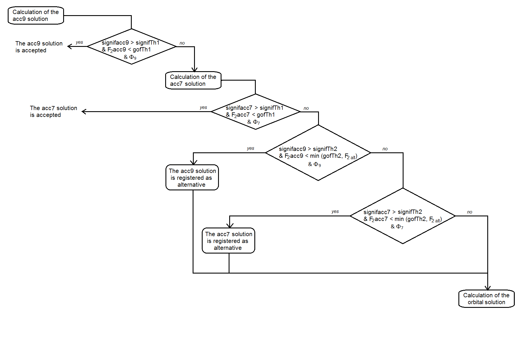
After implementing these additional conditions, the selection of the acceleration solutions followed a process inspired by the preparation of the Hipparcos catalogue, as shown in Figure 7.4: instead of starting with the simplest model, the variable-acceleration solution is derived first. If it is accepted, the constant-acceleration solution is not calculated. Otherwise, it is derived and, possibly, accepted. This strategy allows us to keep the solution that best fits the observations.

The calculation of the astrometric solutions produced 808 992 constant-acceleration solutions and 569 022 variable-acceleration solutions, including alternative solutions. However, only the best of these solutions have been retained after post-processing filtering.

Final selection of the acceleration solutions

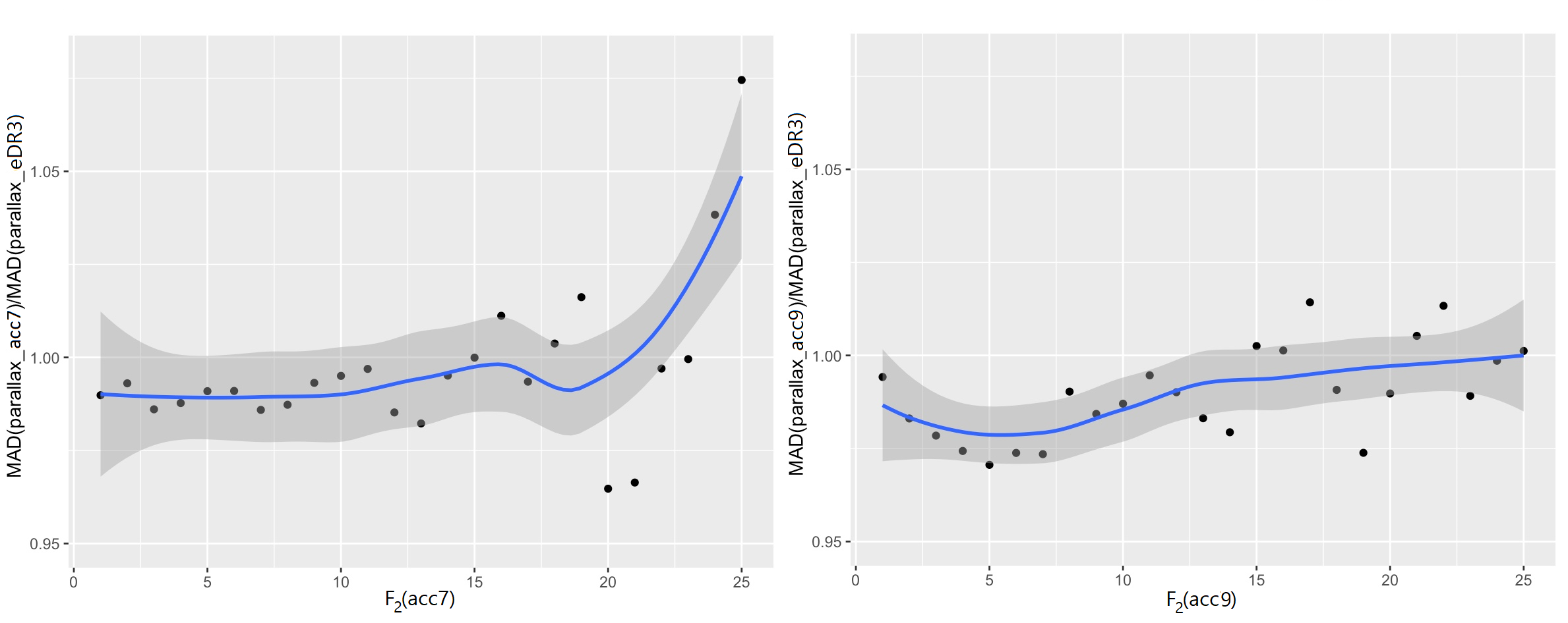
Figure 7.5: Comparison of the width of the parallax distribution obtained with the acceleration solutions over that obtained with the single-star Gaia DR3 solutions. (a): the constant acceleration solutions; the acceleration solutions give more accurate parallaxes as long as $F2\leq 22$ . (b): the variable acceleration solutions; the acceleration solutions win up to $F2=25$ .

After the calculation of all astrometric solutions, and despite the additional selection conditions, it was still considered that the acceleration solutions could be questionable. In addition to the proportion of large accelerations, another criterion was taken into account for setting the thresholds in $F2$ and significance: the quality of the parallax, estimated from the width of the parallax distribution (Figure 7.5). It was found that the parallax of the acceleration solutions was better than that of the single-star solutions of the Gaia DR3 when the significance was larger than 20 for both models and when $F2<22$ for the constant-acceleration model; for the variable-acceleration model, the initial condition $F2<25$ was sufficient.

Thus, the number of solutions retained by the post-processing is finally 246 798 for constant accelerations and 91 227 for variable accelerations.

gaia data release 3 documentation

7.2.4 Acceleration solutions

Calculation of acceleration solutions

Initial selection of acceleration solutions

Final selection of the acceleration solutions