2.4.6 Bias and astrophysical background determination
Author(s): Nigel Hambly
As mentioned previously in Section 2.3.5 concerning bias, on-ground monitoring of the electronic offset levels is enabled via prescan telemetry that arrives in one-second bursts approximately once per hour per device. The processing chain simply analyses these data by recording robust mean and dispersion measures for each burst for each device, and low-order spline interpolation is employed to provide model offset levels at arbitrary times when processing samples from the CCDs. Regarding the offset non-uniformities mentioned previously, the effects are stable on timescales of many months so periodic recalibration takes place every 3 to 4 months and the most recent calibration available for any given processing period is used to correct those features in the data (Section 1.3.3 and Table 1.8). Further details are given in Fabricius et al. (2016) and Hambly et al. (2018).
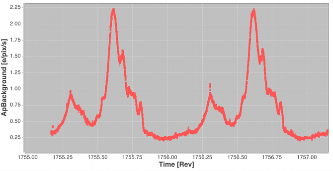
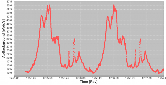
The approach to modelling the ‘large-scale’ background is to use high-priority observations to measure a two-dimensional background surface independently for each device so that model values can be provided at arbitrary along-scan times and across-scan positions during downstream processing (e.g., when making astrometric and photometric measurements from all science windows). A combination of empty windows (VOs; Section 1.1.3) and a subset of leading/trailing samples from faint star windows are used as the input data to a linear least-squares determination of the spline surface coefficients. The procedure is iterative to enable outlier rejection of those samples adversely affected by prompt-particle events (commonly known as ‘cosmic rays’) and other perturbing phenomena. For numerical robustness, the least-squares implementation employs Householder decomposition (van Leeuwen 2007a) for the matrix manipulations. Some example large-scale astrophysical background models are illustrated in Figure 2.11.
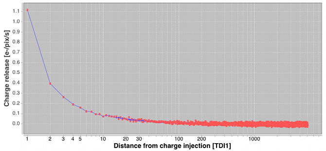
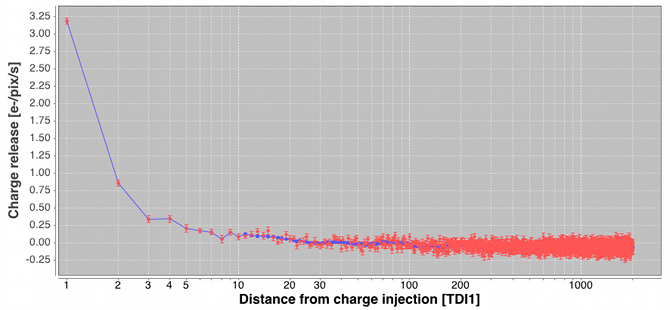
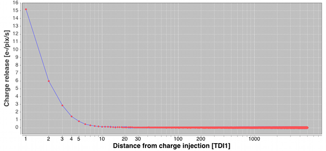
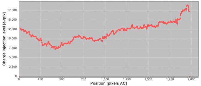
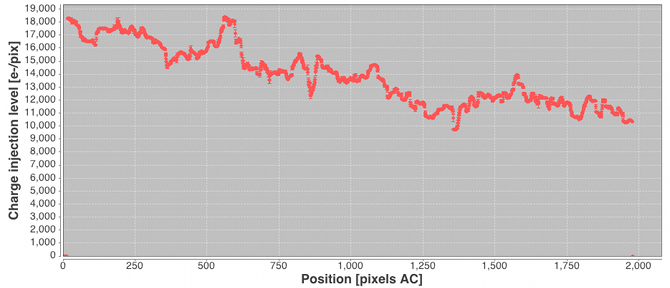
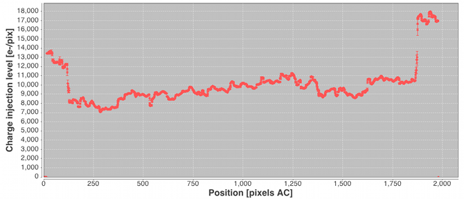
Following the large-scale background determination, a set of residuals for a subset of the calibrating data are saved temporarily for use downstream in the charge release calibration process. Residuals folded by distance from last charge injection are analysed by determining the robust mean value and formal error on that value in each TDI line after the injection. The across-scan injection profile, also determined in a one day calibration employing empty windows that happen to lie over injection lines, is used to factor out the power-law dependency of release signal versus injection level. Note that in this way new calibrations of the charge injection profile and the charge release signature are produced for each processing period. This is done to follow the assumed slow evolution in their characteristics as on-chip radiation damage accumulates (Section 1.3.3). Figure 2.12 shows some example charge release curves typical of those during the Gaia DR2 observation period. Example across-scan charge injection profiles are shown in Figure 2.13.