8.4.2 Additional validation
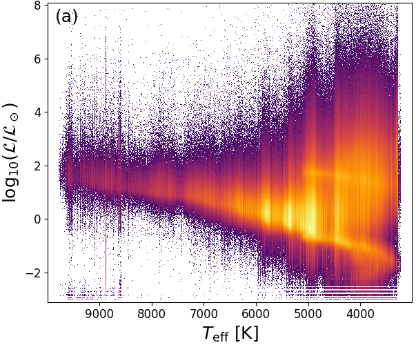
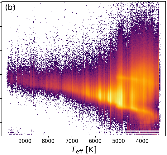
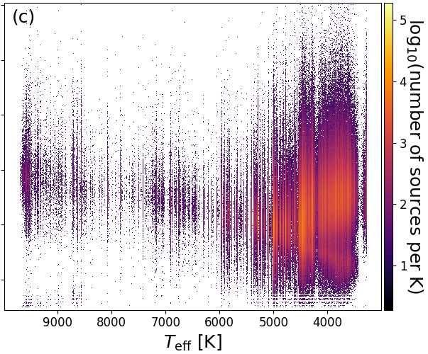
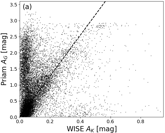
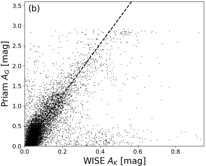
We show the ‘theoretician’s’ Hertzsprung-Russell diagram, vs. , in Figure 8.11a. There are many vertical stripes. When we use the Priam flag values 0100001 or 0100002 (see Table 8.1) to filter for the best data only, Figure 8.11b shows that there are still some stripes left. These are due to the unbalanced distribution in the training sample of ExtraTrees (see Section 8.3.1). Figure 8.11c shows that further vertical stripes are induced by sources which have bad Priam flags.
 |
 |
 |
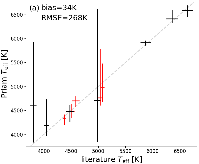
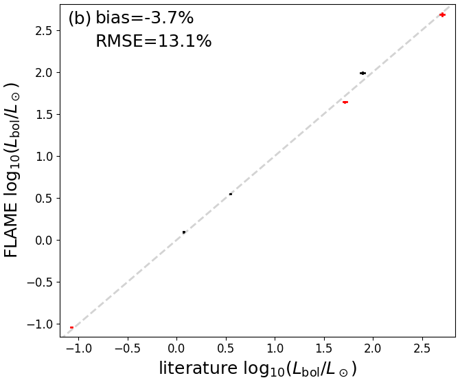
As further validation of both and we investigate the Gaia benchmark stars (Heiter et al. 2015). Unfortunately, most of the 34 Gaia benchmark stars are too bright for Gaia such that we only found 16 of them to have photometry and even only 6 of them to have astrometry in Gaia DR2 (see Table 8.4). Moreover, not all of them are published in Gaia DR2 because some were filtered out due to bad photometry or astrometry. Figure 8.12 shows that the RMS difference in effective temperature is 268K and 13.1% in bolometric luminosity, respectively. This is well within the total error budget of our methods.
| name | Gaia source ID | [mag] | parallax [mas] | Priam [K] | FLAME [] | FLAME [] |
| 61 Cyg A | 1872047223895571456 | 4.71 | – | – | – | |
| 61 Cyg B | 1872046574983497216 | 5.42 | 286.150.06 | |||
| Eri | 5164707970261629952 | 3.37 | – | – | – | |
| Vir | 3736865265439463424 | 2.45 | 30.560.44 | |||
| Sge | 1823067317695767552 | 2.74 | 12.420.36 | |||
| Gmb1830 | 4034171629042489344 | 6.18 | – | – | – | |
| HD107328 | 3701693091058501632 | 4.52 | – | – | – | |
| HD122563 | 3723554268436602368 | 5.86 | – | – | – | |
| HD140283 | 6268770373590148096 | 7.02 | – | – | – | |
| HD220009 | 2661005953843811328 | 4.58 | – | – | – | |
| HD22879 | 3250489115708824064 | 6.52 | 38.200.07 | |||
| HD49933 | 3113219383954556416 | 5.65 | 33.440.09 | |||
| HD84937 | 615943806835727872 | 8.19 | – | – | – | |
| Hya | 3478394889480965120 | 3.17 | – | – | – | |
| Ara | 5945941905576552448 | 4.90 | – | – | – | |
| Leo | 643819484616249984 | 3.42 | 30.650.42 |
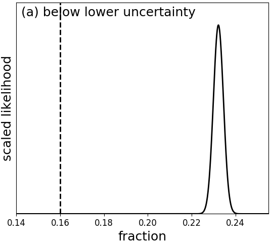
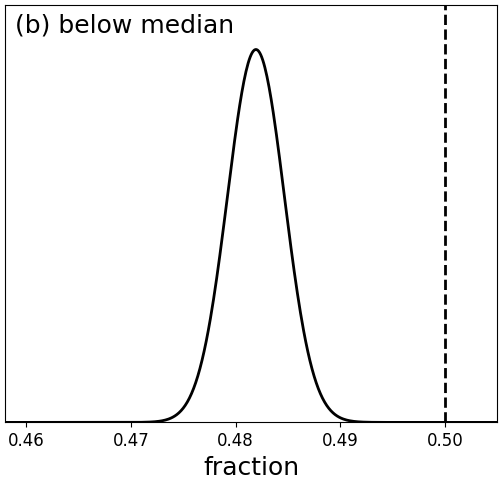
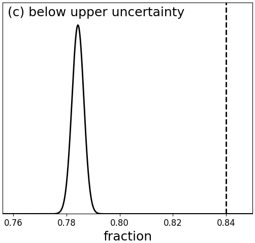
We next investigate the estimate (the median of the ExtraTrees outputs) and the uncertainty estimates, which are 16th and 84th percentiles of the ExtraTrees ensemble (see Section 8.3.1). For 34 231 test stars with literature estimates of , we find that 16 471 (48%) have a median value which is below the literature value. Likewise, we find that for 7 971 stars (23%), the 16th percentile is above the literature estimate, ans for 7 368 stars (22%), the 84th percentile is above the literature value. Figure 8.13 shows that these numbers are inconsistent with 16%, 50% and 84%. At face value, these results seem to suggest that our estimated uncertainty interval is too narrow. However, we need to keep in mind that the literature values we are comparing to also have errors. If we take the estimated literature uncertainties into account, we find in Andrae et al. (2018) that our estimated uncertainties coincide nicely with the actual errors.
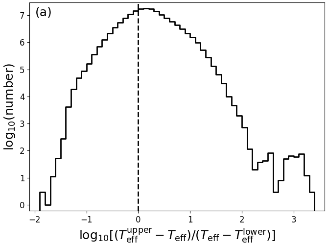
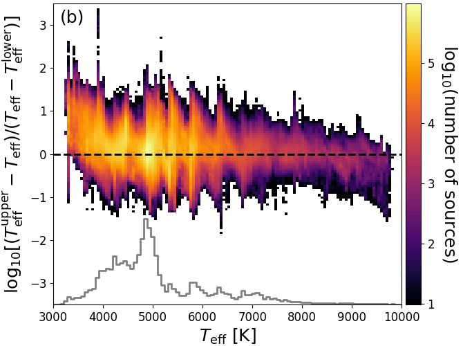
We turn now to the asymmetry of uncertainty estimates for . Figure 8.14a shows the distribution of the asymmetry for all sources with Priam flags 0100001 or 0100002 (see Table 8.1). While for about 57% of sources the upper and lower uncertainty intervals differ by less than a factor of 2, there are also about 2.5% of sources for which the difference is larger than a factor of 10. As it is obvious from Figure 8.14b, boundary effects play a role here: If is close to the lower limit of 3000K, then there is little room left for the 16th percentile, such that the lower uncertainty interval is ‘squeezed’. Likewise, near the upper limit of 10 000K the 84th percentile is restricted, such that there the upper uncertainty interval is also squeezed. However, Figure 8.14b also shows that asymmetries larger than a factor of ten can arise at any other temperature, too. These extreme asymmetries appear to coincide with temperatures that are overrepresented in the ExtraTrees training sample, whereas the asymmetries are more moderate for temperatures where we have little training data.
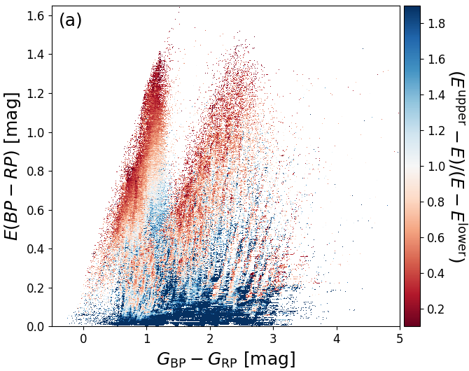
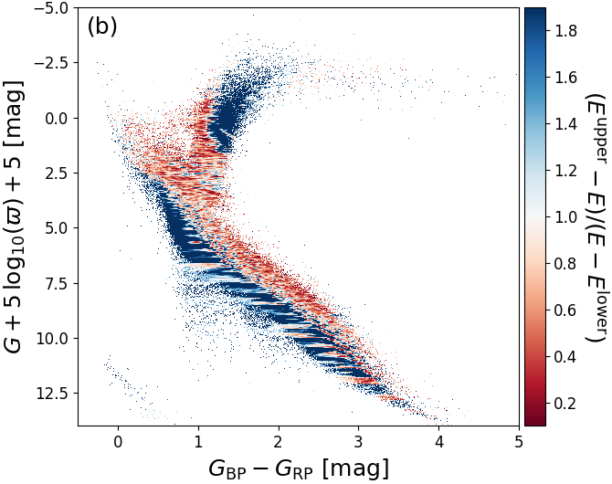
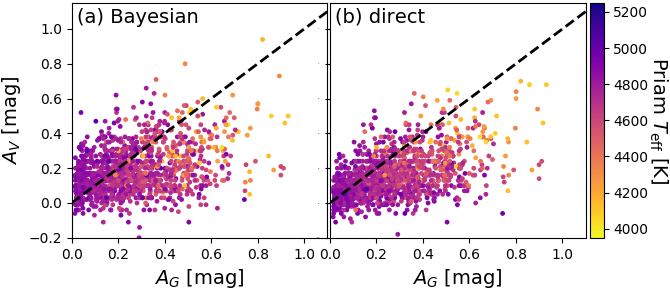
Concerning the degenerate extinction and reddening estimates, Andrae et al. (2018) discuss how degenerate estimates have been identified and filtered out. They only show the results for . Figure 8.15 complements this by also showing the corresponding results for .
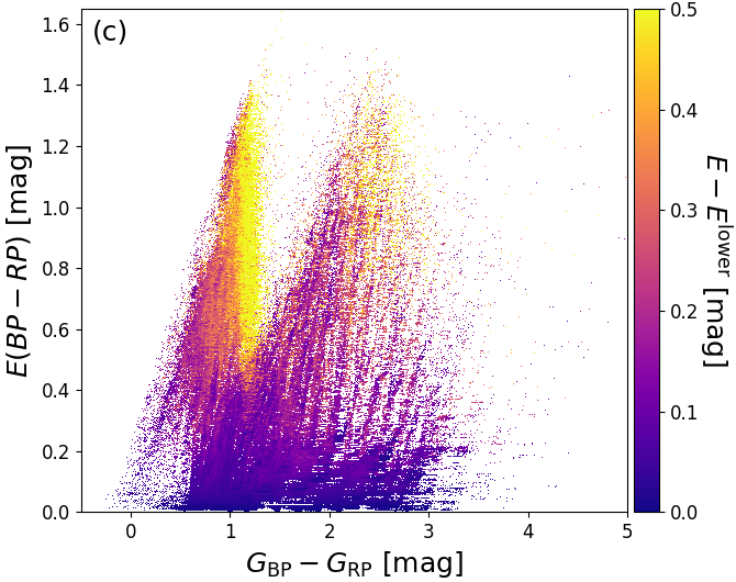
As a demonstration of the usefulness of the additional filtering on extinction that have been applied to Gaia DR2, we investigate the relation between our estimate and the estimate of from APOGEE (Zasowski et al. 2013). We expect an approximate relation of , although this will strongly depend on the adopted extinction law and the intrinsic source SED. Figure 8.16a shows that without the additional filtering there is a prominent group of outliers with low but large . However, these are removed almost completely from the final Gaia DR2 sample, as shown in Figure 8.16b.
 |
 |
As mentioned in Section 8.3.2, there are no literature estimates of or . And since the Gaia passbands are very broad (Jordi et al. 2010) and thus strongly dependent on the intrinsic source SED (see Figure 8.6), it is very hard to meaningfully compare estimates of or to literature estimates of or . Nevertheless, in Figure 8.17 we compare our estimates of to estimates of from Rodrigues et al. (2014). There is a decent correlation, but there is a large scatter in our estimates of . Similar results are seen when comparing to extinction and reddening estimates in the Kepler Input Catalog and estimates from Lallement et al. (2014).
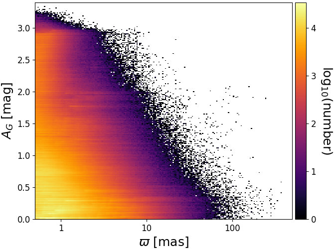
Another important demonstration is that the extinction estimate must approach zero for nearby stars. This is investigated in Figure 8.18. We can see many high-extinction stars below mas, whereas above mas the density profile is an exponential consistent with zero extinction and random noise as explained in Section 6.5 of Andrae et al. (2018). Note that it is not the sharp decline of the maximum above mas, which is only due to a quick decline in number of stars as the parallax increases. Instead, it is the distribution for fixed that changes.
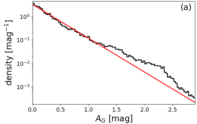
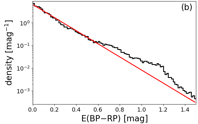
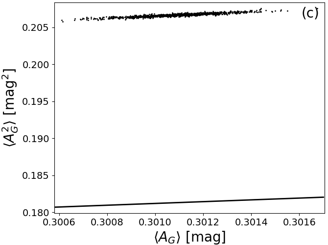
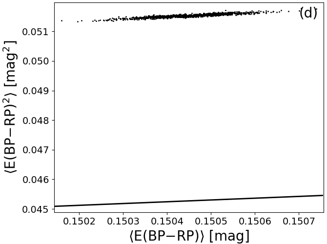
In Andrae et al. (2018), we argue that for high Galactic latitude stars ( ) our extinction and reddening estimates are consistent with an exponential distribution. The exponential would be the maximum-entropy distribution for a non-negative random variate, i.e., the distribution that contains the minimum amount of information (e.g. Dowson and Wragg 2006). This suggests that for high Galactic latitude stars our extinction and reddening estimates are consistent with being pure noise (without systematics). This is further detailed in Figure 8.19. Panels a and b show that for 1.3 mag and 0.6 mag the exponential is a very good fit. However, for larger extinctions and reddenings, there are significant departures from the exponential, with our results having heavier tails than expected. In particular, as pointed out in Dowson and Wragg (2006), the exponential distribution must satisfy the relation between first and second moments. This is tested in Figure 8.19c and d, where we compare the relation to the first and second moments of and , where the moments have been estimated from 1000 bootstrap samples drawn from the sample of high Galactic latitude stars. We can clearly see that the relation for an exponential is not satisfied. More quantitatively, for both, and , the second moment is 14% too large compared to the value expected from the first moment or, alternatively, the first moment is 7% too small compared to the value expected from the second moment. This agrees with our previous observation that the tails of our estimates are too heavy compared to an exponential, because such heavy tails would affect the second moment more than the first. However, our sample may also be contaminated: First, our removal of outliers with degenerate extinction and reddening estimates (see Figure 8.15) is not perfect and outliers that are not caught by the selection criteria from Andrae et al. (2018) would lead to precisely this kind of heavy tails. Second, even at high Galactic latitudes () there are still real dust structures that obtain genuinely high estimates of and , thereby also causing heavy tails. Given these two limitations in our test sample plus the fact that this deviation of 14% from is not very large (although statistically significant), we still conclude that we are largely consistent with an exponential distribution. Consequently, having established the exponential as the maximum-entropy (minimum-information) distribution, we obtain global uncertainty estimates of and from (“standard deviation with respect to ”) given the sample of high Galactic latitude stars.
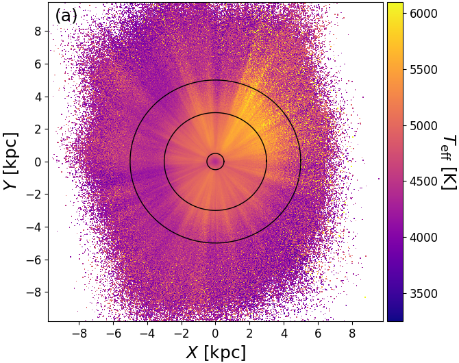
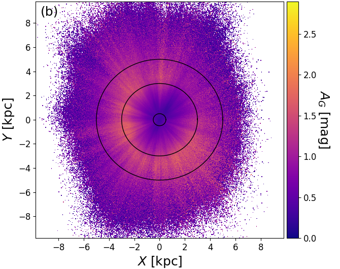
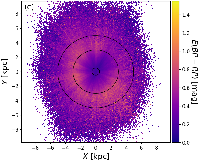
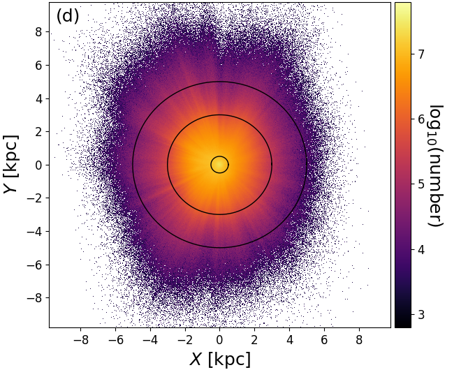
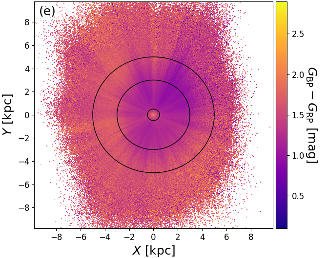
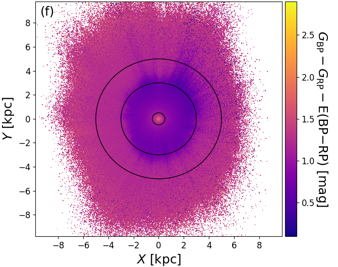
As is shown in Figure 8.20a-c, there are clear ‘fingers of god’ artefacts and ring-like structures in the Apsis results. The fingers of god clearly coincide with high and , which suggests that these are genuine extinction features caused by foreground dust clouds. Comparison to the source density in Figure 8.20d shows that the fingers indeed correspond to lack of sources and comparison to Figure 8.20e shows that the fingers are also systematically redder, as is expected by foreground extinction. The rings are most prominent in Figure 8.20f, where within 0.5 kpc the intrinsic colour is very red, getting bluer around 3 kpc and then turning redder again towards 5 kpc. These rings are most likely due to the dwarf-giant bimodality in the stellar distribution. Faint and cool dwarfs are only detected nearby, thus explaining the red ‘centre’. As we go further out, they become too faint to be detected and only bluer main sequence stars and red giants remain, thus causing the mean colour to become bluer. As we go out even further, also the blue main sequence stars eventually cease to be detectable and we are only left with the luminous red giants, thus causing the mean colour to become redder again. Thus the rings are caused in part by the magnitude limit (G17) of our sample.
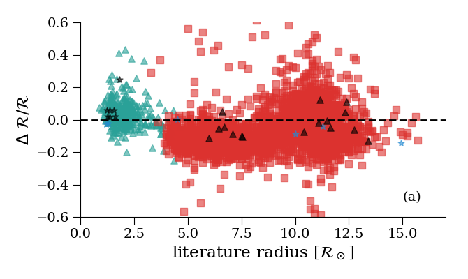
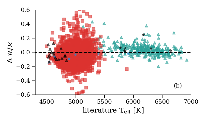
To validate the results for and we compare the derived radii and luminosities with those from a selection of external catalogues, whereby the targets are mostly bright () and nearby ( pc). In Figure 8.21 the FLAME radius is compared to a compilation of asteroseismic and interferometric references as a function of literature radii and . For the less evolved stars ( 3.0 ) the differences are consistent with zero and the scatter is around 7%, consistent also with the radius uncertainties for this range (Andrae et al. 2018). The green triangles represent radii from automatic asteroseismic analysis using scaling relations, where typical uncertainties in the radius can be 5% and the actual values of the radii are rather sensitive to the input (see Chaplin et al. 2014). For this sample we also find a systematic trend in the radii which increases with decreasing . This suggests that the differences in the radii results from the different temperature scales used. The other stars in this less evolved sample range have been studied in much finer detail using interferometry or detailed asteroseismic analysis (black and blue stars). For these better studied stars, we do find much better agreement with the FLAME radii (), with no significant differences as a function of .
The largest sample in Figure 8.21 is that from Vrard et al. (2016), who studied red giants using asteroseismic scaling relations. For the giants, typical uncertainties in the asteroseismic radii are on the order of 7–10% and can also show systematic differences due to the adopted . As explained earlier, we ignore interstellar extinction, and thus we expect the luminosities and radii to be systematically underestimated. This is particularly problematic for giants which are more distant, as extinction could be non-negligible. Figure 8.21 shows indeed that the FLAME radii are slightly underestimated. However, the large scatter is also a result of the differences in the scales, with Priam having values typically cooler than the values used by Vrard et al. (2016).
As with the main sequence stars, the interferometric sample (blue stars) and the giants in NGC 6819 (black triangles), which were studied in much finer detail, show agreement with the FLAME radii to within the 10% level and no trend in their differences as a function of radius or .
 |
 |
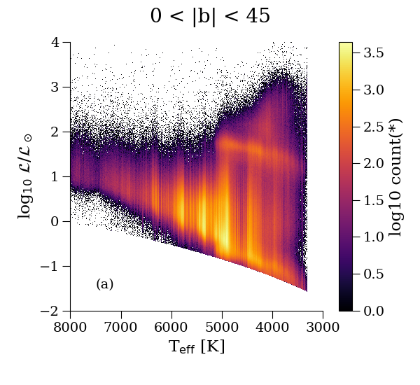
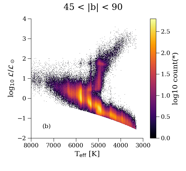
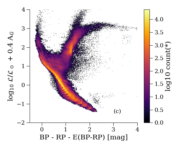
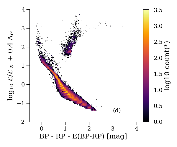
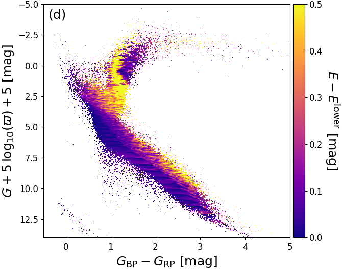
Further validation of the FLAME luminosity is shown using the Hertzsprung-Russell diagrams shown in Figure 8.22. The upper panels exhibit a sharp diagonal cut at the bottom. This is a result of the removal of stars with by the post-processing filtering. It is also evident from panel a (low Galactic latitudes) that where extinction is non-negligible, the and can be underestimated. However, moving to regions of the sky where extinction is much less of an issue (high Galactic latitudes, panel b), we see that the main components of the Hertzsprung-Russell diagram are much more distinct and not contaminated. If we replace the abscissa by the dereddened colour and apply Equation 8.7 to correct for extinction, using , the Hertzsprung-Russell diagrams (lower two panels) show quite narrow main sequence and giant regions, thus validating Priam E(BP-RP).