4.5.5 Analysis of the phase - magnitude relation
Author(s): Alberto Cellino
A key parameter to describe the illumination conditions at the epoch of the observation of an SSO is the so-called phase angle, defined as the angle between the directions to the Sun and to the observer, as measured from the centre of mass of the object. According to its definition, the phase angle is zero when the object is observed in conditions of ideal solar opposition (or in conjunction with the Sun, when it is not evidently observable), and it reaches an upper limit that depends upon the orbit of the object and of the observer. More distant solar system objects can be observed from the Earth, or from the Gaia orbit, only in a narrow interval of possible phase angles, whereas objects approaching or sweeping the inner solar system can be observed over a much wider interval of phase angles. Based on the sky scanning law of Gaia, only very distant Solar System objects can be seen not far from solar opposition whereas, in the case of main-belt asteroids, the interval of possible phase angles has a minimum value around 10 degrees.
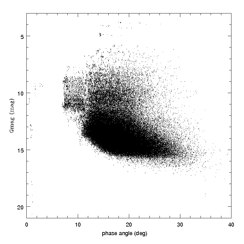
It is known that asteroids tend to become fainter when observed at increasingly large phase angles. In the domain of phase angles covered by Gaia observations, the behaviour consists of a nearly-linear increase of magnitude (normalized to unit distance) for increasing phase angle. It is therefore useful, as a first preliminary check of the Gaia asteroid photometry, to analyze the phase-mag relation. This is shown in Figure 4.33, displaying the whole set of SSO transits, after removal of those not passing the colour-based filter described in Section 4.5.4. The magnitude data shown in Figure 4.33 were obtained after a preliminary conversion of apparent magnitudes into the values corresponding to unit distance from both the Sun and Gaia, using Equation 4.9. It is interesting to see in this plot the presence of a small number of transits of objects seen at small phase angles. These are distant objects, belonging to the Centaur population (Chiron) or to the even more distant population of Kuiper belt objects, including the dwarf-planets Pluto, Haumea and Makemake. Apart from these, the plot shows essentially the behaviour of the asteroid population (dominated by, but not limited to, main belt objects, as explained in Section 4.2.1). A general trend of decreasing brightness for increasing phase angle is seen as expected, but some apparently strange features and discontinuities are also present, and cannot be immediately interpreted in a straightforward way.
Some caveats are immediately important. First, one has to consider that asteroid magnitudes are subject to significant shape-dependent, cyclic variations due to rotation around the spin axis. In classical ground-based studies, one deals normally with full light-curves obtained at different phase angles, and the phase - mag relation is derived by considering only values of magnitude taken at the maximum (or minimum) or each light-curve, in order to avoid to mix together magnitude data corresponding to different cross-sections of the rotating body. Moreover, in ground-based studies data are generally collected during one single apparition of an object, namely during a relatively short interval of time (several weeks), during which the object is seen in a nearly constant geometric configuration, with only the illumination conditions, described by the phase angle, varying with time. In the case of available Gaia data, instead, we deal with sparse photometric measurements taken during a considerable interval of time. The phase - mag relation derived by such data is intrinsically noisy, because it includes measurements taken at epochs corresponding to different illuminated cross-sections, due both to differences of rotation around the spin axis, and to differences of the orientation of the body with respect to the line of sight, if data were taken at epochs sufficiently distant in time. In other words, the phase - mag curves obtained from Gaia transits are contaminated by magnitude variations that are not uniquely due to differences in phase angle.
Moreover, we also have to take into account that at this stage we still do not have in general many transits per object, and those that we have cover often intervals of phase angles that may be fairly small. In other words, an analysis of the phase - mag relation in Gaia DR2 is forcefully still tentative, and it is certain that the achievable results must be considered as very preliminary. However, this analysis has been attempted at this stage, just as an exercise aimed at checking that the currently available Gaia photometric data for asteroids do not exhibit macroscopic anomalies. The analysis considered the available transits for a sample of 8473 objects observed during the interval of interest. For each object, we first computed the conversion from the measured apparent magnitude to the value corresponding to unit distance from the Sun and from Gaia, based on the known values of heliocentric and Gaia-centric distances at each transit. For each object, among all the subsets of magnitudes measured during the same Julian day, generally corresponding to two or more consecutive detections in the two FOV of Gaia, only the brightest recorded magnitude was kept for the analysis, to limit the noise due to different angles of rotation of the object around its spin axis, so mimicking in part the procedures used to exploit full light-curves taken from the ground. At this stage, the rejection filter based on colour data described in Section 4.5.4 was also applied. Transits for which the measured G magnitude had a nominal error of 0.1 mag or larger, and/or the or had abnormal values were discarded a priori. The next step was to discard all objects for which the number of magnitude measurements (after removal of all but one measurement taken during the same Julian day) was less than 6, or the interval of phase angles covered by the observations was narrower than 5 degrees. For each accepted object, a further averaging was done of all the magnitudes obtained in bins of phase angles 1 degree in width (in a very few cases, the latter averaging could lead to accept objects for which the finally averaged transits could eventually cover an interval of phase angles a little smaller than 5 ). Finally, a linear least-squares fit of magnitude versus phase was computed.
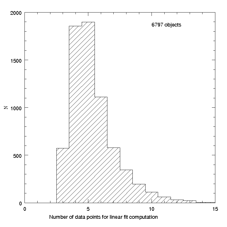
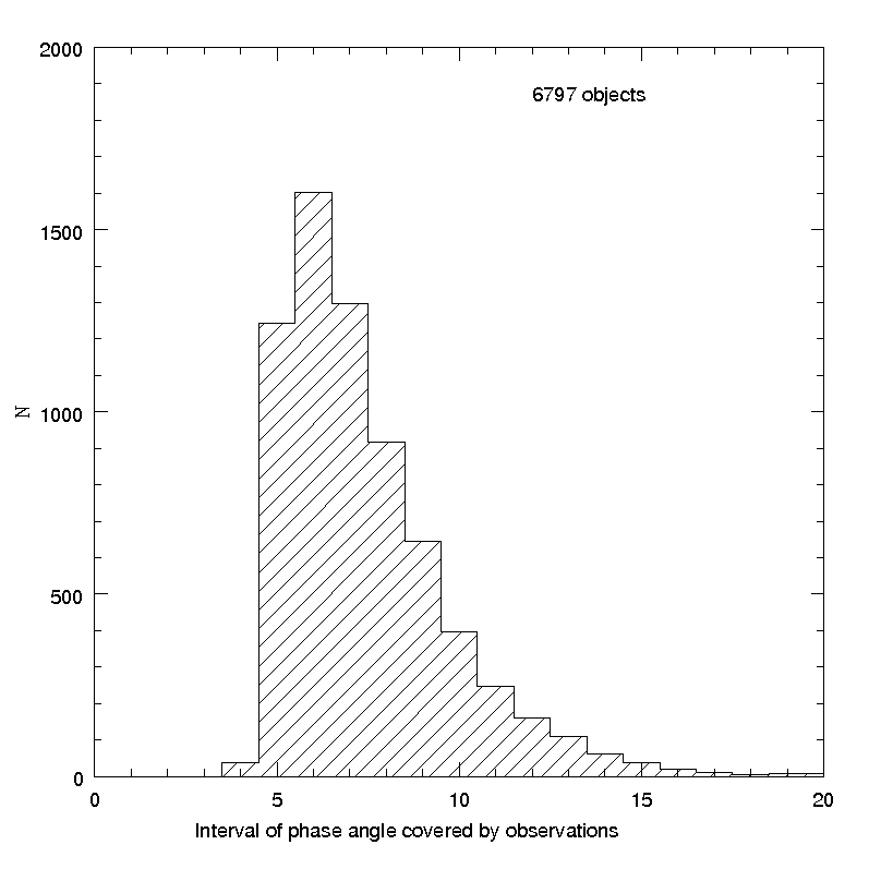
The number of objects satisfying the above criteria was 6797. Figure 4.34 shows the histograms of some parameters of fundamental importance for the analysis, namely the number of magnitude measurements per object and the width of the interval of phase angles covered by the observations of each object. It is easy to see that the number of available data per object is in the majority of cases no larger than 5, and only in a minority of cases the interval of phase angles covered by the observations reaches at least 10 . In these conditions, we cannot expect to obtain linear phase - magnitude relations of a good quality.
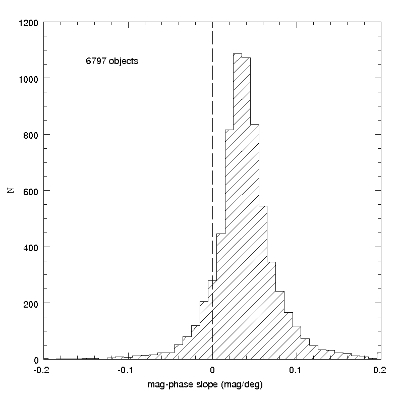
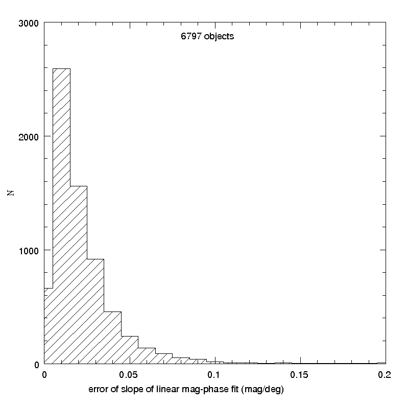
These expectations are confirmed by the results of our exercise. The distribution of the computed linear slopes, and the distribution of the corresponding formal errors, are shown in Figure 4.35. The existence of a non-negligible fraction of aberrant cases, including negative slopes (corresponding to objects for which the brightness seems to increase for increasing phase angle), is well visible. The distribution of slope errors shows that in many cases the resulting linear fits are far from being affected by small uncertainties.
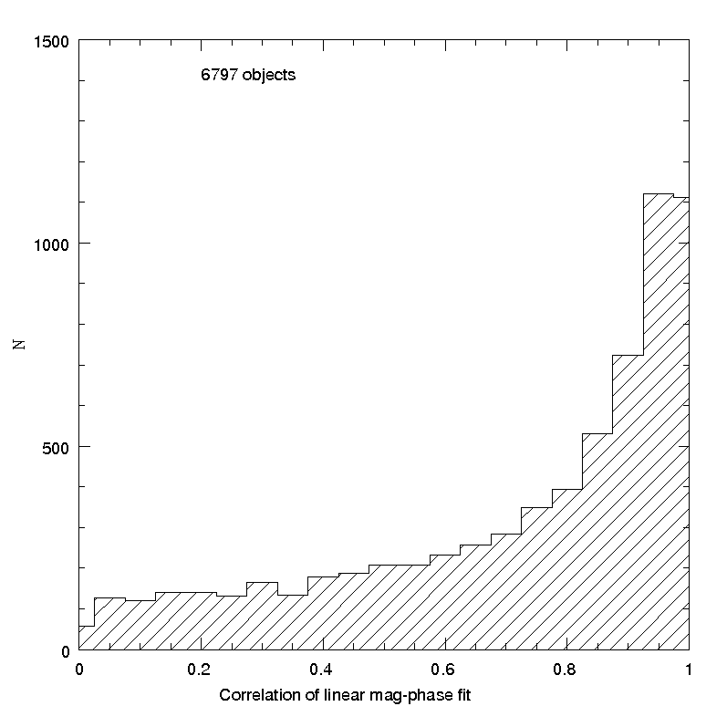
The fact that in many cases the available data cannot be reliably fitted by a linear relation is also shown in Figure 4.36, in which the histogram of the obtained values for the correlation of linear fits are shown. It is easy to see that the distribution peaks at high correlation values, but a very large tail of poor correlation values is also well visible.
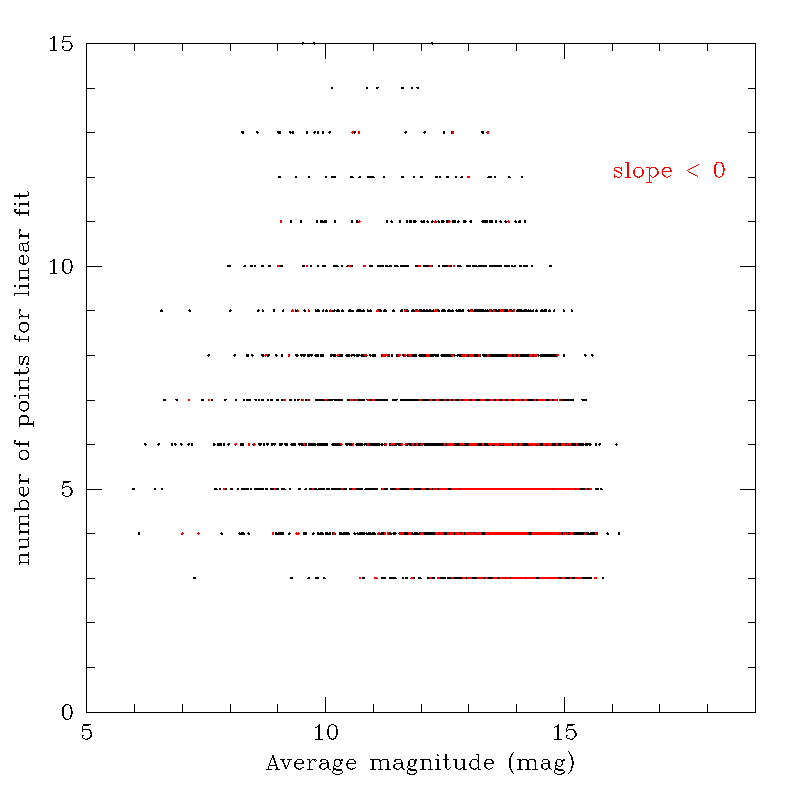
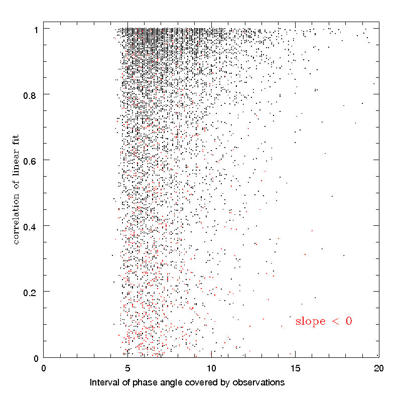
The results confirm therefore the existence of many cases in which it is not possible to produce good linear fits of available phase - magnitude data. This fact, however, should not be overemphasized, because in many cases reasonably good linear fits are obtained, with slopes which are perfectly compatible with those that are typically found from extensive ground-based measurements. In many cases, the aberrant results can be removed by simply imposing strict acceptance criteria in terms of input data quality and quality of the best-fit results. Figure 4.37 shows, as an example, that negative values of the phase - magnitude slope (plotted in red) are mostly found among faint asteroids for which only small numbers of transits are available for computation of a linear fit. In the same plot, it is also evident that negative slopes are preferentially obtained in cases of objects for which poor values of the linear correlation are found, and these are preferentially cases for which the interval of phase angle values covered by the observations is narrow.
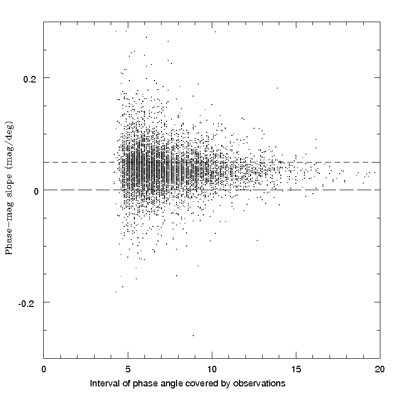
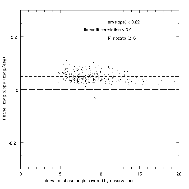
The importance of removing linear fits of bad quality data is also shown in Figure 4.38, in which the computed linear slopes are plotted as a function of the width of the available interval of phase angles. By removing objects for which the number of observations is low, the correlation of the linear fit is bad and the resulting linear slope is affected by large uncertainties, the plot becomes much more acceptable, with a nearly total removal of the cases of aberrant slope values.
Summarizing, we can say that an analysis of the phase - magnitude relation using available SSO photometric data in Gaia DR2 indicates that in most circumstances the available data cover only small intervals of phase angle, and/or the number of observations is too small to produce the clean linear trends that are obtained by using full lightcurve data taken from the ground, and using only the lightcurve maxima to compute the fits. However, even with these limitations, it turns out that in the most favourable cases the objects observed in Gaia DR2 exhibit a phase - magnitude behaviour fully compatible with expectations, taking into account the unavoidable noise produced by using only limited numbers of sparse photometric data.