4.5.2 Quality control of Astrometry
Author(s): Thierry Pauwels, Federica Spoto, Paolo Tanga
Comparing uncertainties with s
 |
 |
 |
 |
 |
 |
 |
 |
 |
 |
 |
 |
 |
 |
During the validation process, we computed the best fitting orbit to Gaia data and the post-fit residuals () to each observation. We could thus check the coherence of the error model with the s. For this purpose it was assumed that the errors on the positions from the orbit are negligible compared to the errors on individual positions, so that the s reflect the real errors on the positions (except for possible systematics that might be present throughout the mission). In order to be able to validate the uncertainties, we separated the s also in a systematic and random part. For the systematic part we took the average of all s of the transit, and for the random part we took the difference between each individual and the average.
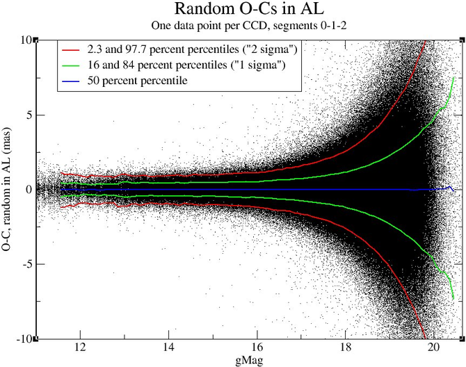
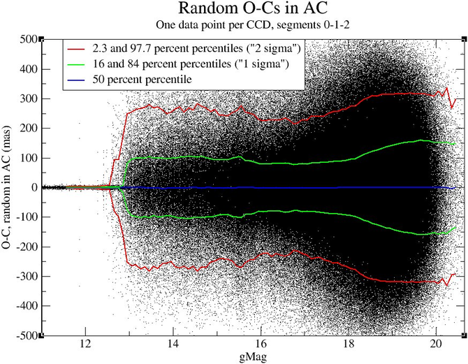
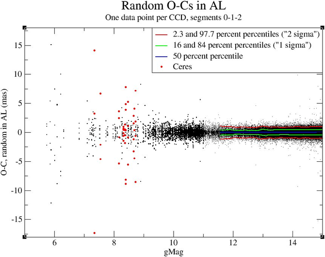
The left panels of Figure 4.21 and Figure 4.22 show the random part of s in AL and AC respectively. As expected, we see that in AL the s increase with increasing magnitude, due to the progressive deterioration in the centroiding performance. For brighter objects ( 16), the s become independent of magnitude, since the errors from centroiding are smaller than those due to the attitude.
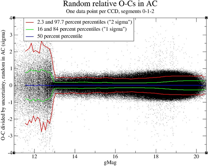
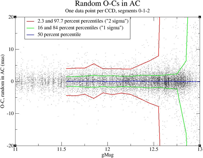
In AC the situation is different. For objects with G13, with 1-D windows, the error comes from the fact that the window centre has been used as an estimate of the position of the object, and it is not dependent on magnitude. Minor variations are present, whose relevance is marginal, whose origin deserves further investigations. Objects brighter than magnitude 13 have 2-D windows (see the left panel of Figure 4.23 for a zoom of Figure 4.22). The situation is similar to AL, where the errors on the attitude dominate, and the s are independent from magnitude.
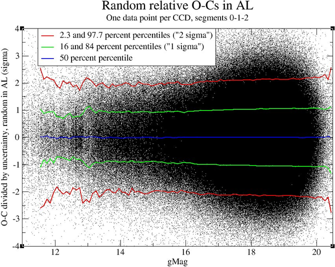
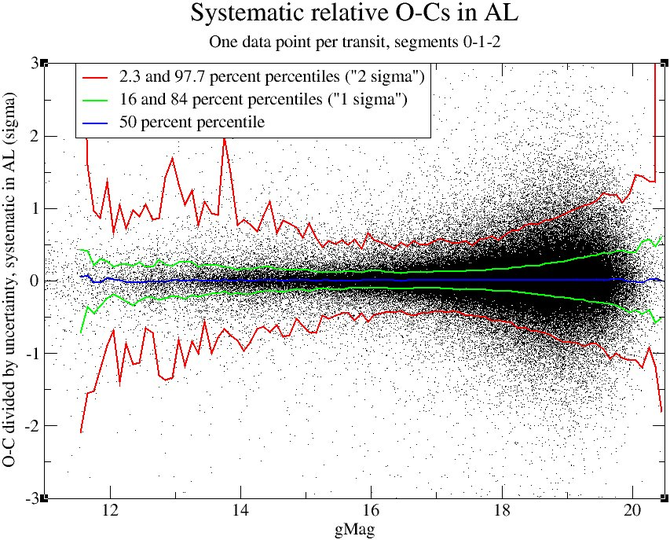
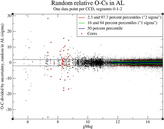
The right panels of Figure 4.21 and Figure 4.22 give the same information, but divided by the computed uncertainties, with the correction , where is the number of positions in the transit after removal of the positions that were rejected. The figures show also the 2.3, 16, 50, 84 and 97.7 percentiles, which correspond to the , , median or mean, 1 and 2, respectively, under the hypothesis that the s follow a Gaussian distribution.
In AL the s behave as expected over the whole brightness range, with the percentiles following almost exactly the values , , 0, and . In AC the situation is again different. For objects brighter than magnitude 13, the behaviour is similar to AL, but for fainter objects the real s are a lot smaller than the computed uncertainties. This is explained by the fact that uncertainties are given as coming from a rectangular distribution over the complete transmitted window, while in reality a majority of objects will be closer to one of the central pixels, as explained in section 4.4.4.
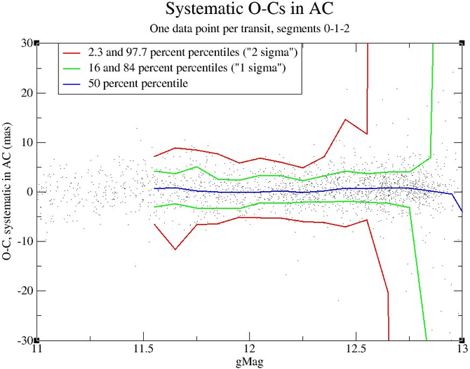
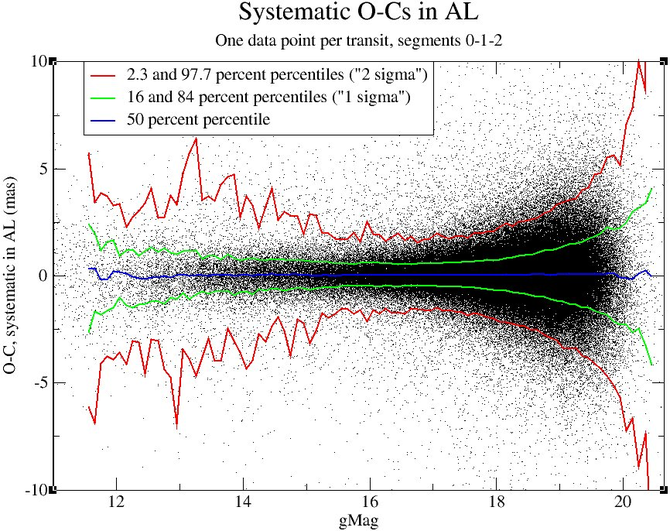
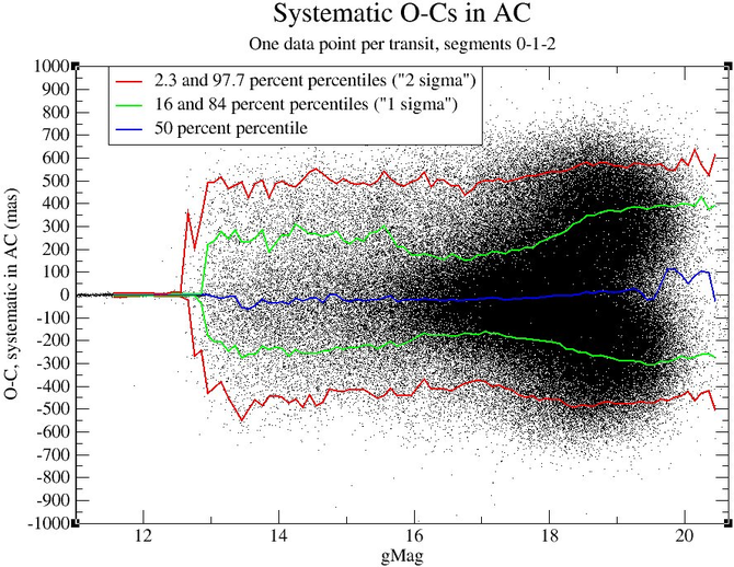
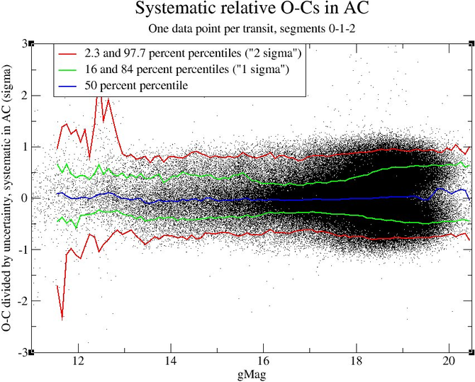
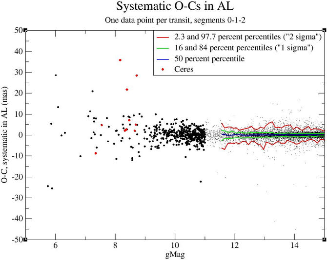
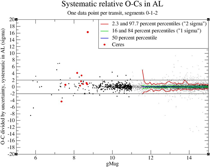
Figure 4.24, Figure 4.25 and the right panel of Figure 4.23 for a zoom on Figure 4.25 represent the same for the systematic errors. Both in AL and AC we see a slightly less good agreement with the error model as the O-C are smaller than expected. This fact indicates that our model for systematic errors is rather conservative. We also note that in AC a bi-variate distribution for faint objects appears (at magnitudes fainter than 18).