4.5.1 Quality control and rejection at CCD level

Only centroids/fluxes obtained from windows with standard characteristics were accepted and transmitted to the following steps of the CU4 processing chain. Windows were required to have normal rectangular shape and all samples of the same window had to have the same integration time. Moreover, windows were processed only if possible intra-field conflicts had been fully resolved and did not go through any kind of truncation. By intra-field conflicts, we mean cases in which images coming from the two FOV of Gaia may receive partly overlapping windows on the focal plane. Finally, windows affected by charge injections were also discarded.

IDT/IDU output data are provided together with a set of parameters summarizing possible problems encountered during the IPD process and the quality of the final result. In some cases, IDT/IDU-derived centroids and fluxes may be included in the database in spite of some anomalies identified during the centroiding process. Typical situations are (1) cases when the maximum number of allowed iterations in the recursive algorithm of maximization of the adopted likelihood function is exceeded. (2) the detection of some illegal input due to charge injection close to the window. (3) other particular problems like cosmic rays. In order to avoid such kind of situations, only IDT/IDU centroiding results for which the relevant quality code indicates a fully successful IPD process were accepted.

It must be noted, however, that no filtering or rejection was done on the basis of the final goodness of fit of the IPD process. The reason is that the signal of a SSO is not expected to be perfectly described by the pure instrumental PSF used by IDT/IDU, mainly due to the SSO residual motion with respect to the TDI charge transfer. As a consequence, the ${\chi }^2$ may well be often worse than in the case of star sources. On the other hand, this fact does not mean necessarily that the values of the centroids and fluxes obtained using only the PSF are completely unreliable, as discussed in what follows.

Biases depending on PSF distortions due to the SSO sources could not be corrected in Gaia DR2. The adopted strategy consisted in rejecting the centroids (and corresponding fluxes) that, within a given probability, could have been affected by a bias larger than the random error due to the photons noise statistics. The aim of this procedure was to avoid, as much as possible, the use of centroids likely affected by some non negligible systematic biases in the following astrometric reduction processing.

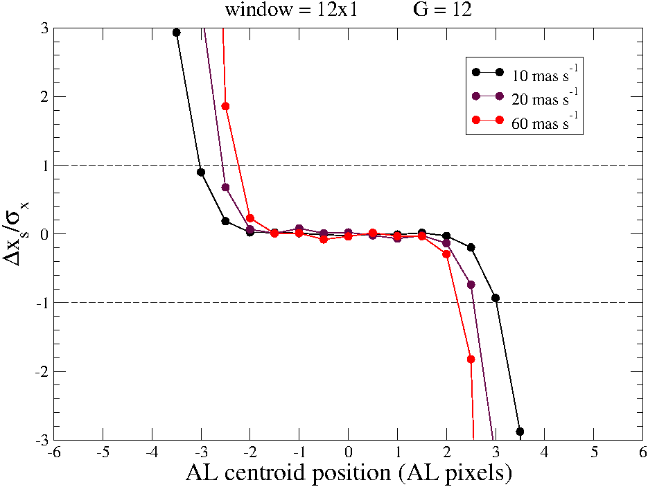
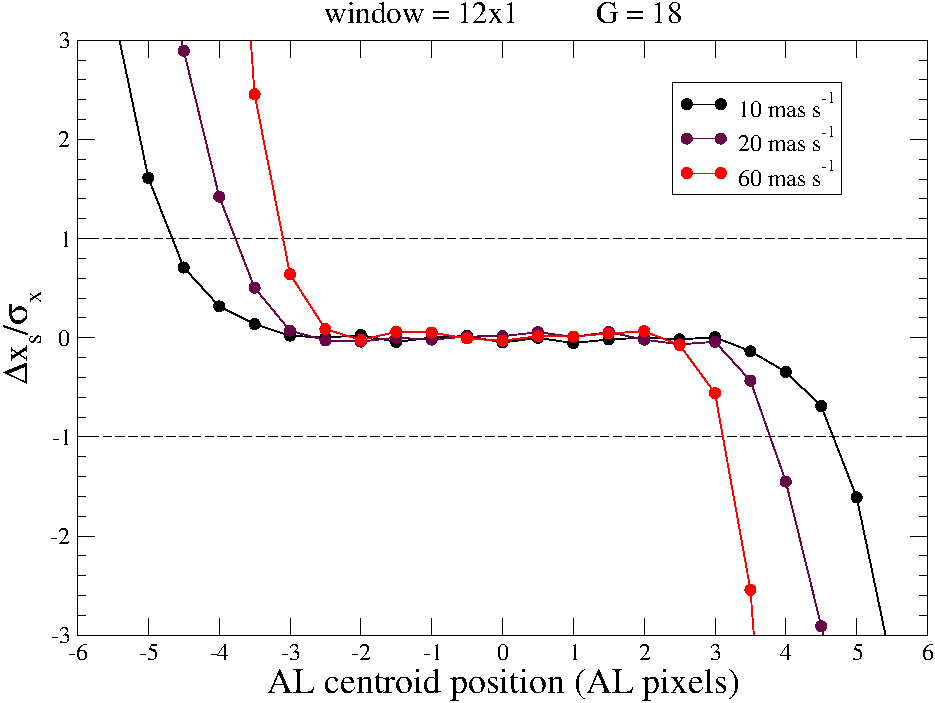
A large set of numerical simulations were performed in order to evaluate the expected centroid and flux bias affecting IPD in a variety of possible situations. In the simulations, nominal PSFs for Solar-type sources were used to model the ${\varphi }_s$ function (for the meaning of the ${\varphi }_s$, ${\mathrm{\Phi }}_s$, $\mathrm{\Delta }{x}_s$ and $\mathrm{\Delta }{f}_s$ symbols used in this paragraph, see Section 4.4.2). Values of resulting $\mathrm{\Delta }{x}_s$ and $\mathrm{\Delta }{f}_s$ were computed for different values of the relevant parameters, namely the window size, the centroid position and the source velocity. Figure 4.20 shows an example of this exercise. Two plots of $\mathrm{\Delta }{x}_s/{\sigma }_x$ versus the centroid position are shown, where ${\sigma }_x$ is the uncertainty in the centroid determination mainly due to photon statistics, which in turn depends on the source magnitude. Two cases for magnitude $12$ and $18$ are shown. It is possible to see how the interval $[-{ℛ}_x,+{ℛ}_x]$ of centroid coordinates (with respect to the window centre) for which depends on source apparent velocity and magnitude. The larger the velocity, the more ${\mathrm{\Phi }}_s$ differs from ${\varphi }_s$ and the larger is the bias, while the interval $[-{ℛ}_x,+{ℛ}_x]$ tends to shrink around zero (${ℛ}_x$ decreases). The fainter is the magnitude, the larger the centroiding error ${\sigma }_x$, therefore the condition corresponds to wider intervals $[-{ℛ}_x,+{ℛ}_x]$ (${ℛ}_x$ increases).

The value ${ℛ}_x$ is a function of the instrument PSF ${\varphi }_s$, the number of along-scan samples $N_x$, the binning $B_x$ (number of pixels per samples), the magnitude of the source $M$ and its along-scan velocity $v_x$. The function ${\varphi }_s$ is not exactly known but it can be approximated on the basis of numerical simulations and nominal payload design. The same for the motion $v_x$, that it is estimated by the IDT/IDU system or it can be constrained by introducing some a priori limits (for example, about $90$% of the Main Belt Asteroids are expected to show an along-scan motion less than $20$ mas/s). The value of the magnitude was estimated on-board by the VPU. In conclusion, from a statistical point of view, we can estimate, for each transit and window, the value ${ℛ}_x$ such that if $x_s\notin [-{ℛ}_x,+{ℛ}_x]$. In such cases, most likely $x_s$ is affected by a bias $\mathrm{\Delta }{x}_s$ larger than its random error due to the photon noise. Whenever this happened, the centroid value $x_s$ was rejected, and the corresponding CCD strip removed from the data processing pipeline.