4.5.3 Photometric variability of SSOs
Author(s): Alberto Cellino, Marco Delbò
The task of finding an effective way to validate a set of SSO photometric data is not straightforward. The reason is that bodies like the asteroids, which constitute the large majority of SSOs observed by Gaia, exhibit a strong photometric variability. The apparent brightness of a SSO depends, at each transit, upon a large variety of parameters. First, and most trivially, the distances from the Sun and from the observer change continuously, and so does correspondingly the apparent magnitude. This can be easily taken into account whenever the positions of the observer and of the target are known. The first step in any analysis of a set of photometric observations of an asteroid is therefore a simple reduction of the recorded apparent magnitude to the value corresponding to unit distance from both the Sun and from the observer, using the simple formula:
| (4.9) |
where and are the reduced and apparent magnitude, respectively, and and are the distances from Gaia and from the Sun, expressed in Astronomical Units. In this, and in the following Section 4.5.4, Section 4.5.5 and Section 4.5.6, both in the text and in the Figures, if not differently specified, the word “magnitude” will always mean . Moreover, it is important to note that we have worked in terms of magnitudes computed at the level of transit, namely after some procedure of averaging of the fluxes recorded by single CCDs during the transit of the object across the Gaia focal plane, according to procedures explained in Chapter 5.
Using magnitudes reduced to unit distance, one can analyze the variation of the brightness of any given object observed at different epochs. This variation is due to a variety of effects, including:
-
1.
The illumination conditions, described in terms of the so-called phase angle, namely the angle between the directions to the Sun and to the observer as seen from the body. The phase angle is zero for ideal solar opposition, a condition which is never met by Gaia observations of asteroids, due to the properties of the sky scanning law of the satellite.
-
2.
The orientation of the body with respect to the line of sight of the observer. This is due to the fact that the shapes of the objects are irregular, and the cross section changes when seen from different directions.
-
3.
The rotation of the object around its spin axis, which continuously modifies the cross section of the illuminated area seen by the observer, again as a consequence of an irregular shape.
-
4.
The role played by the light scattering properties of the surface, which may act in different ways in different observing circumstances. Single and multiple scattering of the sunlight incident onto the surface determine the intensity of the flux measured by the observer, with a complicated dependence upon poorly known surface properties, including albedo, texture and roughness.
Based on the above considerations, and even neglecting some more exotic situations that might occur in principle, it is clear that accurately predicting the expected brightness of an asteroid observed at a given epoch requires knowledge of a number of fundamental physical parameters characterizing the object, including the shape, the spin period, the spin axis orientation, the light scattering properties of the surface (or, at least, a good estimate of the variation of the brightness as a function of the phase angle), and, last but not least, the value of the rotation angle (with respect to some coordinate system) at a reference epoch.
It is also important to note that, in order to compute expected magnitudes with an associated error bar sufficiently small to make useful comparisons with actual sets of photometric measurements, the above parameters must be known with great accuracy. For instance, the knowledge of the rotation period, determined in most cases from ground-based photometric observations carried out several years ago, must be accurate enough to allow us to determine the rotational phase after many thousands of rotational cycles. As a consequence, the rotation period must be known with an accuracy generally not worse than one second of time. Decades of ground-based photometry, mostly at visible wavelengths, have produced a fairly large catalogue of asteroid light-curves, from which the rotation periods have been derived with good accuracy for a data-set of the order of objects. Among them, however, the number of objects observed in a variety of observation circumstances sufficient to derive accurate estimates of the spin axis direction and of the overall shape, derived using complex algorithms of light-curve inversion, is much lower, of the order of some hundreds. In many cases the pole direction estimates are fairly uncertain and the results obtained by different authors may diverge significantly. As for the scattering properties of asteroid surfaces, our current knowledge is extremely limited in all but a few cases.
On the other hand, there are some fundamental properties of the measured fluxes of visible light received from SSOs that can be used to define some fundamental rejection criteria: A first, trivial one is related to the nominal uncertainty of the measurement of the magnitude, as determined by the data reduction pipeline (see the Photometry Chapter in this document). Measurements affected by large nominal errors have been immediately rejected. Photometric errors can be in many cases a consequence of a fundamental problem affecting Gaia observations of SSOs, namely the apparent motion during a transit across the focal plane. As outlined in many Sections of this Chapter, this motion can bring the object close to the border of, or even beyond, its allocated observation window. The consequence can be a considerable loss of flux during the transit, from the astrometric CCD AF1 to AF9. The details depend, of course, on the observing circumstances. Sometimes an object exhibits a very limited motion and remains visible during the whole transit inside its allocated observing window. Sometimes, an object can completely exit from the window before reaching the last astrometric CCDs. Typical situations are shown, as an example, for a tiny, randomly chosen sample of six asteroid transits shown in Figure 4.28, for which the corresponding magnitudes of the objects, determined by the photometric reduction pipeline, are listed in Table 4.2, together with the values of the AL and AC motion, according to ephemerides.
| Transit Id | Asteroid | mag | ( mag) | dAL/dt | dAC/dt |
| mas/sec | mas/sec | ||||
| 51715313735750955 | (2459) Spellmann | 16.5001 | 0.018 | 2.52 | 2.43 |
| 51725151012656516 | (1672) Gezelle | 16.8122 | 0.008 | 0.62 | 2.84 |
| 37293289959334752 | (36) Atalante | 16.2556 | 1.082 | -18.13 | 11.77 |
| 47204317358126290 | (652) Jubilatrix | 16.1868 | 0.097 | -5.48 | 4.29 |
| 51763902126007200 | (1089) Tama | 16.1500 | 0.063 | -3.06 | 21.16 |
| 45597980071694809 | (722) Frieda | 18.8747 | 1.039 | 12.12 | 11.74 |
As can be seen, in some cases the flux is rather constant throughout the transit, but in other cases the average value of magnitude is affected by a large error. This is generally due to a flux loss occurring during the transit, the instant of beginning of the phenomenon being generally related to the speed of the apparent motion, as expected if the flux loss is due to the object progressively drifting to the edge of the observing window. The situation appears sometimes to be more complicated, however. In some cases, the flux recorded by some of the first AF CCDs can be discrepant with respect to the flux recorded by the other AFs. In some situations, it may happen that the flux is not detected at all in some, but not all, AFs, like in the case of the transit of asteroid (722) Frieda shown in Figure 4.28.
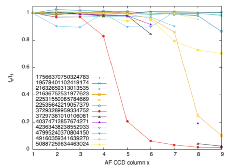
As a consequence of the flux loss, the nominal error of the magnitude determination can increase up to high values. Note that, for any given object, the behaviour can be completely different in different transits, as expected, since each transit corresponds to a different observing circumstance. As an example, Figure 4.29 shows the different behaviour exhibited in 13 different transits of asteroid (36) Atalante. Only in some of the transits of this object, a clear flux loss is observed.
Taking into account these flux loss effects, in Gaia DR2, the choice was to discard all mag measurements having an associated nominal uncertainty worse than 0.1 mag. This corresponds to a maximum permitted value of about 0.1 for the relative error of the flux.
A second acceptance criterion is based on the fact that the colour of the light received from SSOs must be compatible with the properties expected for scattered sunlight. This allows us to define possible acceptance criteria based on available colour data and a comparison with the colours measured for stars of solar type. This will be described in Section 4.5.4. We can already anticipate at this stage that applying a filter based on nominal magnitude error and measured colour indexes led us to discard from the Gaia DR2 results all the so-called “bronze” transits, those having poorly calibrated BP/RP fluxes. Only the so-called “gold” and “silver” transits, corresponding to the best-calibrated sources, have been retained by the procedures of SSO photometry validation.
Another general property that can be used to make some validation check, is the fact that the brightness of SSOs tends to decrease when observations are made at increasingly large phase angles. This property can be used as a validation criterion, but, as will be explained in Section 4.5.5, there are practical complications that make this test to be subject to significant uncertainties in many cases.
Eventually, the most stringent validation checks must rely on a comparison of measured versus predicted magnitudes for sets of observations of the same object obtained at different epochs. As discussed above, the computation of predicted magnitudes requires an accurate knowledge of many physical parameters. In most cases, we have not a sufficient knowledge of all of them, and we are forced to rely on information concerning the spin period and the direction of the spin axis, only, while fine details of the shape, including for instance the presence of concavities, are not accurately known. Moreover, also the surface light scattering properties are affected by quite large uncertainty. In these situations, the results of validation procedures must be taken with some care, since the error bars in the corresponding magnitude predictions are unavoidably not small. On the other hand, this kind of test is potentially possible for a relatively large number of objects, provided that the number of available Gaia observations is sufficiently large to allow us to obtain some reasonable set of O-C values.
In principle, the best possible validation test must consist of comparisons between expected and measured magnitudes for a small number of objects for which our knowledge of their physical parameters is extraordinarily accurate, being based on in situ measurements carried out by space probes. The problem is that the number of asteroids visited by space probes is still extremely low. For what concerns Gaia DR2, only two objects, the main belt asteroids (21) Lutetia and (2867) Šteins, satisfy these criteria.
In the next subsections, the procedures of validation adopted for SSO photometry, based on the principles expressed here in most general terms, are presented in deeper details.