5.3.3 Geometric Calibration

Author(s): Francesca De Angeli

Since each CCD has a different position on the focal plane and the focal length of each telescope is slightly different, the propagation of the position of the window can be imprecise causing an imperfect centring of the observed source inside the window. In BP/RP observations, these shifts in the AL direction can affect the wavelength calibration and must be estimated.

The correspondence between pixels and wavelengths is provided by the BP and RP dispersion functions, that are defined with respect to the position of a reference wavelength. The location in the sample space of this reference wavelength can change for different transits because of diverse reasons: the source might have a significant AL motion or the on-board window propagation may not be very accurate. The reference wavelength position can be predicted starting from the source astrophysical coordinates, the satellite attitude and the focal plane geometry.

For a set of observed spectra of sources with similar spectral type, the observed location of the reference wavelength is expected to be the same, except for the effects of non-perfect centring of the window, and it can be estimated in the following way: the spectra are first scaled to the same integrated flux and then aligned using cross-correlation to find an initial adjustment in sample position and flux; this adjustment is then refined by fitting a spline to all spectra observed in the same calibration unit and then using that as a reference spectrum to fit second-order corrections to the alignment parameters for that calibration unit. After this second alignment, a reference spectrum is generated from all spectra from different calibration units. This reference spectrum is finally fitted to evaluate the sample position of the reference wavelength within the actual sampling.

The differential corrections that need to be applied to the nominal focal plane geometry are then modelled from the difference between the observed and predicted locations of the reference wavelength. For more details see Carrasco et al. (2016).

The application of these differential corrections is done on all spectra and it consists of two steps:

• •

  Differential geometric calibration application: defines for each observed spectrum the AL location of the reference effective wavelength. This is referred to as the observed arbitrary reference sample.

• •

  Differential dispersion calibration application: converts the observed sample AL positions into the pseudo-wavelength system. An attempt was made to calibrate the differential dispersion functions as a small correction to be applied to the nominal ones. However, these corrections resulted to be quite small and probably related to contamination effects. For this reason they were not applied in the Cycle 03 processing, where instead the nominal dispersion functions were adopted.

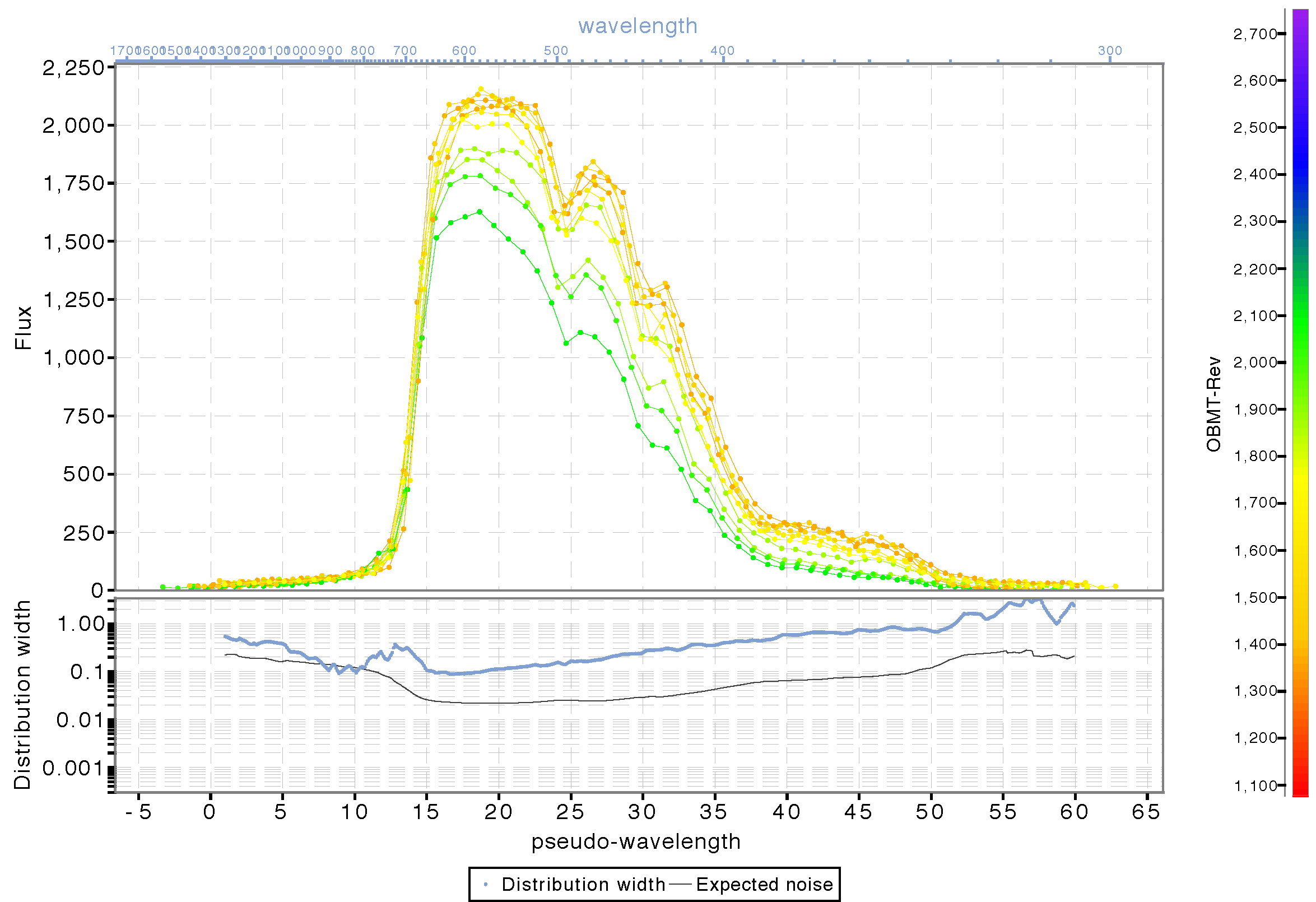
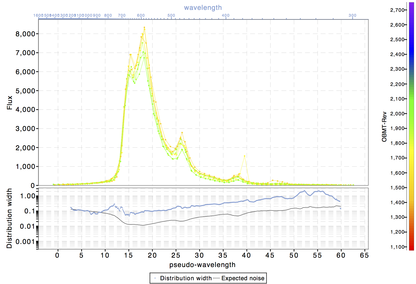
Figure 5.7 and Figure 5.8 show two examples of epoch (BP) spectra. Figure 5.7 is for a SpectroPhotometric Standard Source (see Section 5.6) while Figure 5.8 is for an emission line source. Here all epoch spectra have been calibrated for background, differential dispersion and geometry achieving a good alignment of the main features. Clearly no flux calibration has been applied, and contamination effects (varying with time) are quite evident and still present in the spectra. These will be taken care of in downstream processing.