5.3 BP/RP spectroscopic processing 5.3.4 Internal Calibration 5.3.6 Catalogue of BP/RP spectra in Gaia DR3

5.3.5 External calibration

Author(s): Paolo Montegriffo

The two main tasks of the external calibration are: i) provide an instrument model to allow for a physical interpretation of the BP and RP mean spectra, and ii) transform the mean spectra to fully calibrated (flux and wavelength) spectral energy distributions.

The external calibration is based on the following main assumptions:

•

all differential effects across the focal plane (including variations with time) are completely accounted for by the internal calibration;
•

the internal reference system is uniquely defined for all sources, independently from source colours and magnitudes;
•

the internal reference system can be represented by an instrument model that is close to the physical instrument at an arbitrary position on the focal plane.

Instrument model

The dispersed image of a point-like source in the data space can be expressed as:

\Im(u,w)=P_{\tau}\,\int\limits_{0}^{\infty}n_{p}(\lambda)\,P_{\lambda}\left(u-% u_{d}(\lambda),w\right)\,R(\lambda)\,{\rm d}\lambda

(5.3)

where:

•

$u$ is the continuous coordinate in the along scan (AL) direction;
•

$w$ is the continuous coordinate in the across scan (AC) direction;
•

$P_{\tau}$ is the telescope pupil area in units of $m$ ;
•

$n_{p}(\lambda)$ is the source photon flux distribution (SPD) in units of $photons\,s^{-1}m^{-2}nm^{-1}$ ;
•

$P_{\lambda}(u,w)$ is the effective monochromatic point spread function (PSF) at wavelength $\lambda$ ;
•

$u_{d}(\lambda)$ is the dispersion function;
•

$R(\lambda)$ is the overall instrument response function.

This model assumes that i) the dispersion of the prism is perfectly aligned with the AL direction, and ii) charge transfer inefficiency (CTI) effects can be neglected. The BP and RP spectra are originated by collapsing the 2D image along the AC direction, thus giving:

n_{e}(u)=P_{\tau}\,\int\limits_{0}^{\infty}n_{p}(\lambda)\,L_{\lambda}\left(u-% u_{d}(\lambda)\right)\,R(\lambda)\,{\rm d}\lambda

(5.4)

where

•

$n_{e}(u)$ is the internally calibrated mean spectrum in units of $e^{-}s^{-1}$ ;
•

$L_{\lambda}(u)$ is the effective monochromatic LSF at wavelength $\lambda$ .

The classical approach of deriving an instrument response by computing a ratio between the observational spectra and the corresponding SPD over a limited number of featureless calibrators cannot be applied here because of the large LSF width compared to the wavelength scale of response variations. As a consequence LSF and dispersion relation must be derived together with the instrument response. This can be achieved in principle using an arbitrarily large number and variety of standard stars (sources with known spectral energy distribution) by tuning the model till a match is obtained between the model prediction and the corresponding observational mean spectra.

However, the stringent criteria set to select reliable flux calibrators (see Section 5.6) led to a selection of stars spanning a limited range in astrophysical parameters, whose SED shapes are not sufficiently independent from each other, and hence leave a relevant number of instrument components undetermined. This limitation is mitigated in two ways: i) by building the instrument model upon a nominal model based on the pre-launch knowledge of the actual instrument, and ii) by employing in the calibration process a large set of additional sources that escape the severe selection criteria adopted for the standard flux calibrators, but exhibit narrow emission lines in their spectra (possibly) all along the covered wavelength range: candidate sources of this kind are QSOs, Be stars and other $H_{|}\alpha$ emitters, Wolf-Rayet stars etc. For the Gaia DR3 a total of 211 such sources have been selected, including 188 QSO from the SLOAN survey, 17 young stellar objects from the XSHOOTER database and 6 emission line sources from STELIB (Le Borgne et al. (2003)). Most of these objects have SEDs only partially covering the Gaia wavelength range: this limitation had consequences on the processing strategy, as described in Section 5.3.5.

LSF model

The monochromatic LSF is obtained by integrating $P_{\lambda}$ in the AC direction. The LSF model is based on a linear combination of the product of two sets of basis functions modelling respectively the AL and the wavelength dependency; these bases have been derived with the Generalised Principal Component Analysis (GPCA) on a large set of theoretical LSFs simulated for the nominal instrument. The framework for PSF/LSF simulations, as developed by Lindegren (Lindegren (2006)), was applied to the present case of the BP/RP spectra calibration, and is described in detail in the technical note Montegriffo (2017).

Theoretical PSFs were computed with an accuracy in the AC direction of $1\%$ up to $\pm 24.6$ pixel from the centre, and the final wavelength grid contains 100 points distributed between $288.4$ and $1153.6$ nm. A total number of 5000 sets of PSF were randomly generated; for each set, a corresponding set of monochromatic LSFs was obtained by summing the PSFs along the AC direction and multiplying by an appropriate scaling factor. Each LSF is then considered twice by reversing the AL axis in order to preserve the intrinsic AL symmetry of the problem.

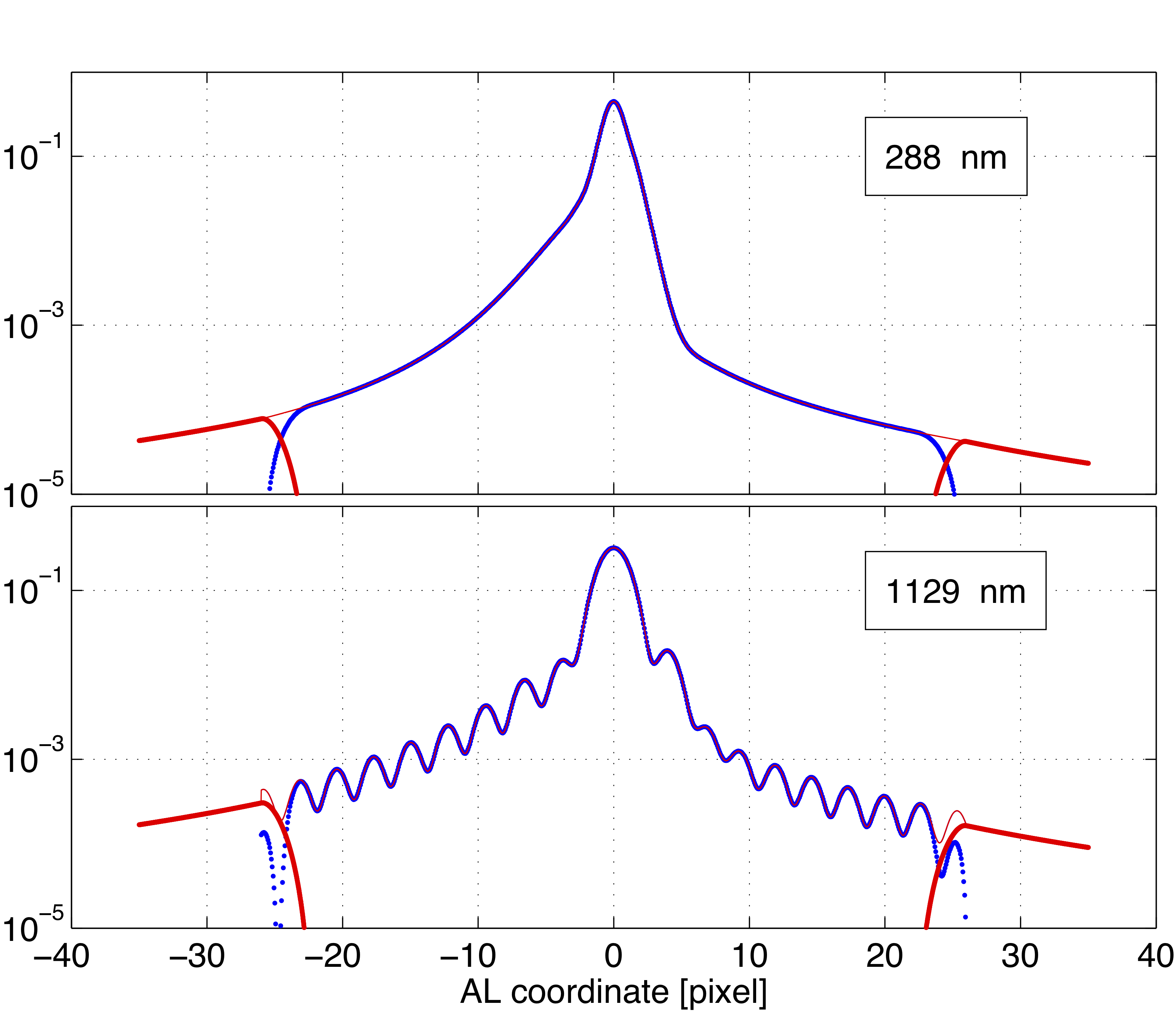
However, such LSFs only span a limited AL interval of $\pm 26$ pixel, therefore a proper model for the wings was derived and applied also in order to correctly normalise the LSFs. The wings for polychromatic and quasi-monochromatic LSF were modelled by a tail function which is strictly zero for $u<\alpha$ , decreases as $u^{-2}$ for $u>\beta$ thus reproducing the expected behaviour of a true LSF, and is a fourth-degree polynomial in the interval $[\alpha,\beta]$ , where $u$ is the AL coordinate in pixel, and $\alpha=22$ , $\beta=26$ are the $u$ values at wich the tail function joins the LSF. To make the analytical LSF representation continuous at $u=\pm\beta$ a proper scaling factor is applied. As an example, the reconstruction of a LSF at $\lambda=288$ nm and $\lambda=1129$ nm is shown in Figure 5.9.

Figure 5.9: Blue dots represent the simulated model of the LSF, and red dots show the two scaled tail functions; the semi-analytical LSF model is the sum of these two components. The top panel refers to $\lambda=288$ nm, the bottom panel to $\lambda=1129$ nm.

GPCA algorithm is able to preserve the spatial locality of pixels into an image by projecting the images to a vector space that is the tensor product of two lower-dimensional vector spaces. Each simulated LSF is arranged in a matrix whose columns are the monochromatic LSFs sampled on a given $u$ grid; the mean LSF $\overline{L}$ is computed and subtracted from each LSF, and the residuals are arranged in a stack of 10000 matrices which are decomposed through GPCA into a 2D set of bases designed by two matrices $U$ and $W$ modelling respectively the dependence of LSF in sample and wavelength spaces. The $i^{th}$ numerical LSF can be approximated as:

L_{i}\approx U\cdot D_{i}\cdot W^{T}+\overline{L}

(5.5)

or, in extended notation:

L(u_{i},\lambda_{j})=\overline{L}_{u_{i},\lambda_{j}}+\sum_{m=1}^{\ell_{1}}% \sum_{n=1}^{\ell_{2}}d_{m,n}\cdot U_{i,m}\cdot W_{j,n}

(5.6)

The above relation represents the implemented model for the LSF representation: it is 2D-interpolated to continuous variables $(u,\lambda)$ by 1D-interpolation of U and W bases separately. The interpolation function for the U bases must satisfy the ’shift invariant sum’ condition, i.e. preserve the underlying function normalisation independently from the sub-pixel position of the sampling grid: the most suitable interpolation method is given by the S-spline representation described in Section 3.3.5. The interpolation for the right basis functions W is achieved with a cubic spline. A complete description of the model can be found in Montegriffo (2017).

Dispersion model

For each field of view, dispersion functions are provided for the centre of each CCD in the form of the coefficients $A_{i}$ of the expansion:

AL(\omega)-AL(\omega_{ref})=\sum_{i=0}^{N}A_{i}\omega^{i},

(5.7)

where

•

$AL(\omega)$ denotes the AL image position in mm (in the Y FPRS direction),
•

$\omega=1/\lambda$ in $nm^{-1}$ denotes the inverse wavelength, and
•

$\omega_{ref}=1/440~{}nm^{-1}$ for BP and $1/800~{}nm^{-1}$ for RP.

The AL position in pixel units can be obtained by dividing Equation 5.7 by the pixel size of a CCD in the along-scan direction $P_{AL}$ .
The mean instrument dispersion function model is defined by:

u_{d}(\lambda)=\sum_{k=0}^{N_{u}-1}d_{k}\cdot\left[\frac{1}{P_{AL}}\sum_{i=0}^% {N}A_{i}\frac{1}{\lambda^{i}}\right]^{k}

(5.8)

where

•

$u_{d}(\lambda)$ denotes the AL image position in pixel units;
•

the model parameters $d_{0}$ and $d_{1}$ represent respectively the wavelength zero-point and scale: the zero-point is by construction the AL position corresponding to the reference wavelength. The nominal values assumed are $d_{0}=30$ , and $d_{1}=1.0$ and zero for any higher order term for both XP instruments.

This dispersion model defines the origin of the monochromatic LSFs as a function of wavelengths (see Equation 5.4). However, the origin of the LSF does not necessarily coincide with its centroid, because in general the LSF is not symmetric, its shape can change with the wavelength and hence introduces some degeneracy between the chromaticity and the dispersion (Lindegren (2006)). This degeneracy does not affect the instrument model because the dispersion model and the LSF origin are consistently defined. However, for a physical interpretation of the data it is necessary that the dispersion relation provides the centroid of the monochromatic LSF as a function of wavelength. This dispersion relation is provided as a lookup table where at each wavelength $\lambda$ the centroid $u_{0}$ is computed using the Tukey’s bi-weight function by solving the non-linear equation:

\int\limits_{-\infty}^{\infty}L(u_{0}+u,\lambda)\,w(u/s)\,{\rm d}u=0

(5.9)

for $s=2.7$ , where:

w(z)=\left\{\begin{array}[]{l@{\quad}l}z\,\left(1-z^{2}\right)^{2}\quad&{\rm if% }~{}|z|<1\\ \quad\\ 0\quad&{\rm otherwise}\end{array}\right.

(5.10)

The dispersion curve for BP and RP is available from the DR3 area in the Gaia Cosmos portal.

Response model

The response model is built as the combination of a model for the nominal response with a parametrised cut-off $R_{Nom}(\lambda)$ and a distortion model $R_{d}(\lambda)$ to account for the deviations with respect to the current response

R(\lambda)=R_{Nom}(\lambda)\times R_{d}(\lambda)

(5.11)

The nominal photonic response for XP instruments is modelled as the product of the following quantities:

R_{Nom}(\lambda)=T_{0}(\lambda)\,\rho_{att}(\lambda)\,Q(\lambda)\,T_{p}(\lambda)

(5.12)

where

1.

$T_{0}(\lambda)$ is the telescope (mirrors) reflectivity;
2.

$\rho_{att}(\lambda)$ is the attenuation due to rugosity and molecular contamination of the mirrors;
3.

$Q(\lambda)$ is the CCD QE;
4.

$T_{p}(\lambda)$ is the prism transmittance curve which includes filter coating on their surface.

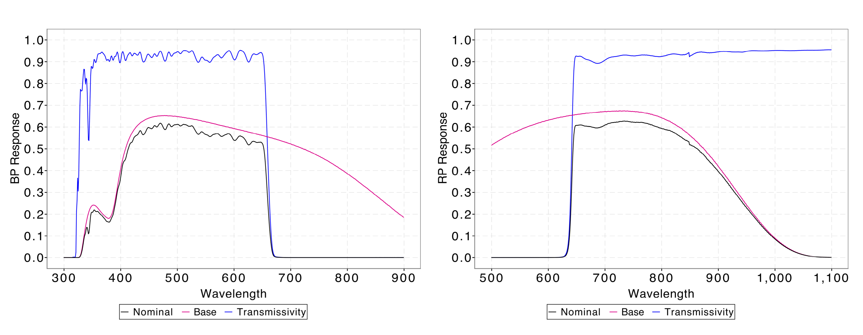
Figure 5.10: BP and RP response components: the black line is the nominal response, the blue line is the photometer transmittance and the red line is the response curve without the photometer transmittance component.

Figure 5.10 shows the nominal curves with an highlight on the photometer transmittance contribution to the overall curves. All these quantities were measured by Airbus DS during on-ground laboratory test campaigns. However, the filter wavelength cut-ons and cut-offs in the prism transmittance curves change over the focal plane due to uneven thickness of the prism coating producing bandwidth non uniformity: the expected variation is of about 3 nm in the position of the BP cut-off and about 2 nm in the position of the RP cut-on (hereafter for convenience cut-off will be used for both instruments). Moreover, combining measurements taken all over the focal plane results in a mean instrument passband with smeared cut-offs. To account for these effects the prism transmittance curve is modelled as follows:

T_{p}(\lambda)=T_{p}^{\dagger}(\lambda)\times R_{cut}(\lambda;\mu,\sigma)

where $T_{p}^{\dagger}(\lambda)$ is the tabulated transmittance curve provided by Airbus DS truncated right before and after the cut-off wavelength for BP and RP, respectively:

T_{p}^{\dagger}(\lambda)_{BP}=\left\{\begin{array}[]{l@{\quad}l}T_{p}(\lambda)% \quad&~{}{\rm for}~{}\lambda<640nm\\ \quad\\ T_{p}(640nm)\quad&~{}{\rm for}~{}\lambda\geqslant 640nm\end{array}\right.

(5.13)

T_{p}^{\dagger}(\lambda)_{RP}=\left\{\begin{array}[]{l@{\quad}l}T_{p}(\lambda)% \quad&~{}{\rm for}~{}\lambda>647nm\\ \quad\\ T_{p}(647nm)\quad&~{}{\rm for}~{}\lambda\leqslant 647nm\end{array}\right.

(5.14)

and $R_{cut}(\lambda;\mu,\sigma)$ is a parametric curve based on the Gauss error function and its complementary function:

R_{cut}(\lambda;\mu,\sigma)=\left\{\begin{array}[]{r@{\quad}l}\frac{1}{2}~{}% erfc\left(\frac{\lambda-\lambda_{co}-\mu}{\sigma_{co}+|\sigma|}\right)\quad&~{% }~{}{\rm for~{}BP}\\ \quad\\ \frac{1}{2}~{}\left(1+erf\left(\frac{\lambda-\lambda_{co}-\mu}{\sigma_{co}+|% \sigma|}\right)\right)\quad&~{}~{}{\rm for~{}RP}\end{array}\right.

(5.15)

where $\lambda_{co}$ represents the nominal cut-off wavelength ( $667.9$ nm for BP, $631.0$ nm for RP), and $\sigma_{co}$ represents the nominal cut-off slope ( $4.71$ for BP, $4.0$ for RP). The parameter $\mu$ controls the wavelength position of the cutoff while the parameter $\sigma$ sets the steepness of the cutoff slope. When the two parameters are set to zero the nominal transmittance curve is reproduced to a relative accuracy better than $0.5\%$ .

Figure 5.11: BP and RP photometer transmittance models: the blue dotted lines represent the photometer nominal transmittance curves, the red lines represent the curves $T_{BP}^{\dagger}$ and $T_{RP}^{\dagger}$ given by Equation 5.13 and Equation 5.14 respectively. The black lines are the transmittance models of Equation 5.3.5 for two different values of $\sigma$ parameter ( $\sigma+\sigma_{co}=5$ for solid black line, $\sigma+\sigma_{co}=20$ for dotted black line). The quantity $\mu-\lambda_{co}$ is set equal to 700nm for the BP model (*left panel*) and to 600nm for the RP model (*right panel*).

Figure 5.11 gives a visual representation of the proposed photometer transmittance model: the nominal transmittance model from GPDB (dotted blue lines) is compared to the $T_{f}^{\dagger}$ models of Equation 5.13, Equation 5.14 and to two different realisations of the $T_{f}^{*}(\lambda)$ model obtained by setting the quantity $\mu-\lambda_{co}$ respectively to 700 for BP and 600 for RP and setting the quantity $\sigma+\sigma_{co}$ to 5 (black solid line) and to 20 (black dotted line). These parameters values have been chosen as mere examples to illustrate the model behaviour.

The distortion model in Equation 5.11 is implemented as the exponential of a linear combination of basis functions in the sample space:

R_{d}(\lambda)=\exp\left(\sum\limits_{i=0}^{n_{R}}r_{i}\,R_{i}(u_{d}(\lambda))\right)

(5.16)

where $u_{d}(\lambda)$ is the nominal dispersion relation. The basis functions used for Gaia DR3 are spline functions of the $2^{nd}$ order.

SED reconstruction

The internally calibrated instrument model can be expressed as:

n_{e}(u)=P_{\tau}\int\limits_{0}^{\infty}\,\mathrm{L}(u,\lambda)\cdot R(% \lambda)\cdot n_{p}(\lambda)\,{\rm d}\lambda

(5.17)

where the kernel $\mathrm{L}$ is a combination of the LSF and dispersion models. We define the effective SPD $n^{*}_{p}(\lambda)$ as the product between the source SPD and the instrument response:

n^{*}_{p}(\lambda)=R(\lambda)\cdot n_{p}(\lambda)

(5.18)

The previous integral equation can be used to estimate the effective SPD $n^{*}_{p}(\lambda)$ given the mean spectrum $n_{e}(u)$ sampled on some pseudo-wavelength grid, then the effective SPD is represented in some parametric form, e.g. a linear combination of a proper set of basis functions $N_{i}(\lambda)$ :

n^{*}_{p}(\lambda)\approx\sum_{i=0}^{N-1}s_{i}~{}N_{i}(\lambda)

(5.19)

Substituting Equation 5.19 into Equation 5.17 leads to:

n_{e}(u)\approx P_{\tau}\sum_{i=0}^{N-1}~{}s_{i}\int\limits_{0}^{\infty}\,% \mathrm{L}(u,\lambda)\cdot N_{i}(\lambda)\,{\rm d}\lambda

(5.20)

that can be rewritten as:

n_{p}(u)\approx\sum_{i=0}^{N-1}~{}s_{i}T_{i}(u)

(5.21)

where

T_{i}(u)=P_{\tau}\int\limits_{0}^{\infty}\,\mathrm{L}(u,\lambda)\cdot N_{i}(% \lambda)\,{\rm d}\lambda

(5.22)

This equation shows that, since the observables are available in sample space and not in wavelength space, the choice of an orthonormal set of basis $N_{i}(\lambda)$ for SED representation does not guarantee that the corresponding instrument-transformed set $T_{i}(u)$ represents as well an orthonormal reference system. Furthermore, Equation 5.17 is a Fredholm integral equation of the first kind, which is generally difficult to solve because the problem is intrinsically ill-conditioned: there are many solutions which satisfy an integral solution slightly perturbed from the original one (the observed spectrum $n_{p}(u)$ is affected by noise).
However, the current representation of the internally calibrated mean spectra described in Section 5.3.4 is based on a linear combination of Hermite functions roughly centred on the observed spectra:

n_{p}(u)\approx\sum\limits_{i=0}^{N-1}\,b_{i}\,\varphi_{i}\left(\frac{u-u_{0}}% {a}\right)

(5.23)

where $u_{0}\sim 30.0$ is the centre of the spectra in the AL coordinate system, and $a$ is a scaling factor to match the width of the observed spectrum with the natural width of the Hermite functions. The similarity between Equation 5.23 and Equation 5.21 suggests the possibility to define a set of functions $\phi_{i}$ such that:

\varphi_{i}\left(\frac{u-u_{0}}{a}\right)=P_{\tau}\int\limits_{0}^{\infty}\,% \mathrm{L}(u,\lambda)\cdot\phi_{i}(\lambda)\,{\rm d}\lambda

(5.24)

These functions $\phi_{i}$ are the instrument-deconvolved versions of the bases used for the mean spectra representation: hereafter they will be called inverse bases. With this set of functions it is then possible to reconstruct externally calibrated SEDs using the same set of coefficients $b_{i}$ provided by the internal calibration for the representation of mean spectra: mean spectra and externally calibrated SEDs can then be sampled to some pixel or wavelength grid by simply changing the set of bases used:

n_{p}(u)\approx\sum\limits_{i=0}^{N-1}\,b_{i}\,\varphi_{i}\left(\frac{u-u_{0}}% {a}\right)

n_{p}(\lambda)\approx\sum\limits_{i=0}^{N-1}\,b_{i}\,\phi_{i}(\lambda)\cdot% \frac{1}{R(\lambda)}

(5.25)

The advantages of this approach are:

•

minimum impact on archive storage requirements;
•

the inversion process is made just once within DPAC calibration activities;
•

the instrument inversion process is not applied to measured mean spectra, but instead to analytic functions that are noise-free;
•

a simple tool can be provided to end-users to reconstruct sampled mean spectra either in the internal system or in absolute quantities.

Equation 5.17 shows that the effective SPD represents the observational spectrum smeared by the LSF and transformed to the pseudo-wavelength space, preserving the basic features of the observational spectrum. Therefore, each right inverse basis of Equation 5.24 is best modelled by the use of the same family of functions that represent the left bases, i.e. a linear combination of Hermite functions with a proper scaling factor and the same centre:

\phi_{i}(\lambda)\approx\sum\limits_{k=0}^{M-1}\,h_{ik}\,\varphi_{k}\left(% \frac{u_{d}(\lambda)-u_{0}}{b}\right)

(5.26)

The complete description of the method used to derive the inverse basis parameters $h_{i}{k}$ can be found in Montegriffo et al. (2023).

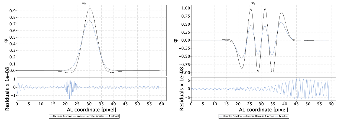
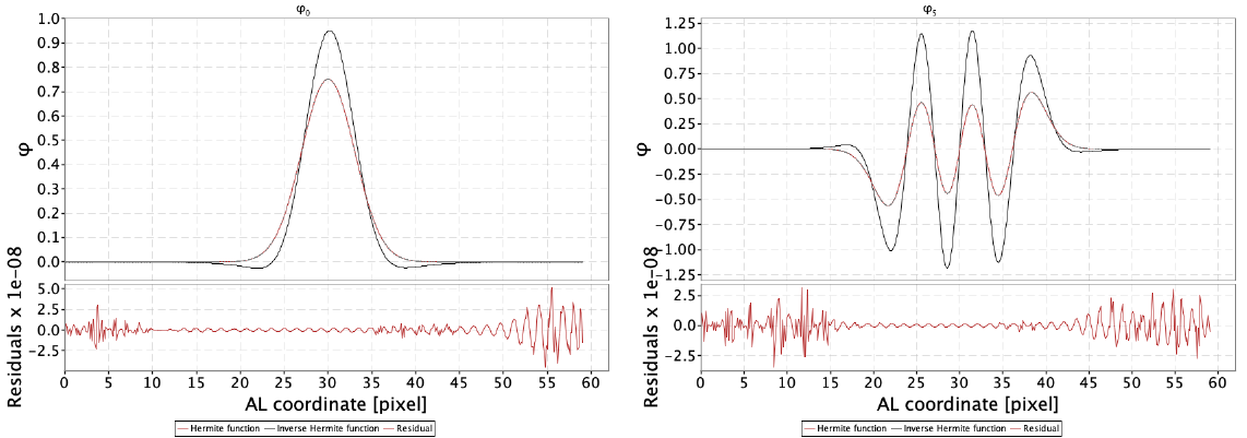
Figure 5.12: Blue/Red lines represent the Hermite function of order 0 (*left*) and 5 (*right*); black lines represent the corresponding inverse functions. In each box the bottom plot represents residuals between the original Hermite function and the reconstructed one. The inverse functions have been modelled using 79 and 87 basis functions for BP (*Top*) and RP (*Bottom*), respectively, and the same scaling factor of the Hermite function.

Figure 5.12 show as an example the $0^{th}$ and $5^{th}$ order Hermite functions and the corresponding inverse bases for BP (Top panels) and RP (Bottom panels) as well as the relative numerical residuals in the reconstruction of the original Hermite function.

As explained in Section 5.3.4 the mean spectra representation has been optimised to concentrate most of the information in the first coefficients, so to provide an efficient way to cope with noisy spectra by truncating the latter terms. This optimisation is realised by a rotation of the Hermite bases by the use of a square orthogonal matrix. The inverse basis function method is not affected by this optimisation as long as the same rotation is applied to the inverse bases.

As can be seen in Equation 5.25 the reconstructed SED depends on the inverse of the response function, therefore to limit errors in the reconstruction the sampling grid can be safely limited to the range $[330,650]$ nm for BP and $[635,1050]$ nm for RP. The two partially overlapping spectra are merged into a single distribution by computing a weighted mean in the overlapping region $[635,650]$ nm with the weight $w_{BP}$ and $w_{RP}$ defined as:

w_{BP}(\lambda)=1-\frac{\lambda-635}{650-635}

(5.27)

w_{RP}(\lambda)=1-w_{BP}(\lambda)

(5.28)

Processing

Optimisation of model parameters is achieved by minimising in a least squares sense a $\chi^{2}$ based cost function:

\chi^{2}=\textbf{r}^{T}\cdot W\cdot\textbf{r}

(5.29)

where r represents the vector of residuals between the observations and the model values, and $W$ is the matrix of weights which is equal to the inverse of the covariance matrix.

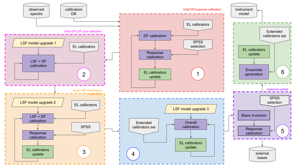
Figure 5.13: Scheme of the external calibration processing.

The optimisation process is carried out using an implementation of the Differential Evolution Algorithm (DEA) as described by Storn and Price (1997). Due to the complexity of the model, great care has been taken to avoid as much as possible local minima in the $\chi^{2}$ space, especially in the first steps of the processing. The adopted strategy has been to begin the first iterations with a simplified version of the model (lower number of parameters and symmetric LSF), and progressively increase complexity as far as convergence was achieved. The general processing scheme is outlined in Figure 5.13 where six different stages are identified: 1) initialisation of the dispersion relation and the large scale modifications of the nominal response; 2) modelling of the interactions between dispersion and LSF core (chromaticity effects); 3) modelling of chromaticity variation with wavelength; 4) modelling of LSF wings; 5) modelling of fine structures in the response model; 6) final overall optimisation and generation of the ensemble of models. Table 5.2 summarises the number of parameters for BP and RP instrument models at different stages of the processing.

Table 5.2: Number of parameters at different stages of the processing for BP and RP instrument models.

	Stage	1	2	3	4	5	6
Dispersion		2	2	3	3	3	3
LSF	BP	(0, 0)	(4, 1)	(4, 2)	(7, 3)	(7, 3)	(7, 3)
	RP	(0, 0)	(4, 1)	(4, 2)	(4, 2)	(4, 2)	(4, 2)
Response	BP	8	8	8(+2)	8(+2)	26(+2)	26(+2)
(+cutoff params)	RP	8	8	8(+2)	8(+2)	23(+2)	23(+2)

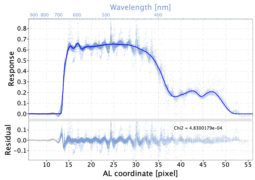
Each optimisation cycle consists of $3\sim 4$ thousand DEA iterations, each one involving 50 walkers (different realisations of model parameters, initially distributed randomly around the starting parameters set), that are eventually stopped when the individual costs from the walkers converge to a common value. The parameter set with the lowest cost is used to initialise the following optimisation cycle and the procedure is repeated till convergence in parameter values is achieved, thus switching to the following stage. In the first stage only a selection of featureless SPSS is used, the response cut-off parameters are kept fixed to the nominal values and the cost evaluation is done avoiding the cut-off regions, while the dispersion relation is fitted using emission line (EL) calibrators. Since EL sources are not reliable flux calibrators (they include variable objects), a grey calibration is applied at each iteration: the input SPD of each EL source is scaled by a parameter that is evaluated to minimise the squared residuals between the current model prediction and the corresponding observational mean spectrum. Stages 2 and 3 are used to initialise the modelling of LSF, while a full optimisation is performed in the fourth stage. In stage 5 the basis inversion process is performed. Inverse bases are used to reconstruct the effective SPD for SPSS; by dividing effective SPD by the source SPD it is possible to trace the overall instrument response as shown in Figure 5.14.

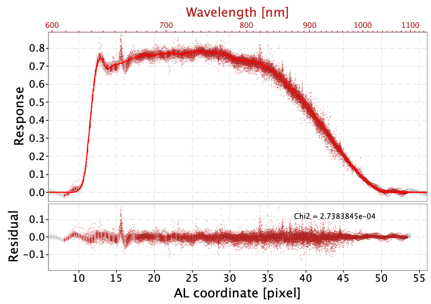Figure 5.14: For each SPSS it has been computed the ratio $R_{eff}$ between the reconstructed effective spectrum $n_{p}^{*}(\lambda)$ from Gaia observations, for BP (*blue*) and RP (*red*), and the corresponding SPD $n_{p}(\lambda)$ . Blue/Red lines represent the response component $R(\lambda)$ of the instrument model plotted as function of AL sample. The top axes represent the corresponding wavelength scale in $n m$ . The bottom plots show the residuals between $R_{eff}$ and the model $R(\lambda)$ .

Two aspects are worth noticing:

•

the signature left in the data by Balmer lines ( $H_{\beta}$ , $H_{\gamma}$ , $H_{\delta}$ in BP, $H_{\alpha}$ in RP) and some Paschen lines (in RP beyond $820~{}nm$ ) are clearly visible: this is due to the error in LSF modelling causing systematic differences in the profile of the absorption lines;
•

a wavy pattern with a well defined spatial frequency is present in the residuals, clearly visible in the BP data while in the RP case the data look more noisy.

It is not fully understood whether the wavy pattern originates from wiggles in the mean spectra (De Angeli et al. (2023)). We have used this data to upgrade the instrument response distortion model by increasing the number of spline knots to model the wiggles especially in the range [500, 800] nm, taking care to exclude the signatures due to absorption lines (the response model must not be a function of any source astrophysical parameter). The model curves represented in the plot have been computed after this upgrade. The final location of spline knots for the BP and RP response models is given in Table 5.3.

Table 5.3: AL location of the knots used for the spline representation of the response distortion for BP and RP models shown in Figure 5.14.

knot	BP	RP	knot	BP	RP	knot	BP	RP	knot	BP	RP
0	15.8	12.8	6	21.0	18.0	12	38.5	29.0	18	45.0	49.0
1	16.7	13.3	7	22.0	19.0	13	40.0	30.5	19	46.0
2	17.6	13.8	8	27.5	20.0	14	41.0	32.0	20	47.5
3	18.3	14.3	9	32.0	26.0	15	42.0	34.0
4	19.0	15.0	10	34.5	27.5	16	43.0	40.0
5	19.7	16.5	11	36.7	29.0	17	44.0	47.0

The last stage is used to create the ensemble of models: the DEA solver is run on the last instrument model till parameter relaxation is achieved (typically after $\sim 400$ iterations), then all the 50 walkers are saved into the database. While the walker that achieves the lowest cost is selected to represent the instrument model, the ensemble is needed to estimate the uncertainties in the simulated spectra, which are especially useful for other CUs to derive source astrophysical parameters.

Results

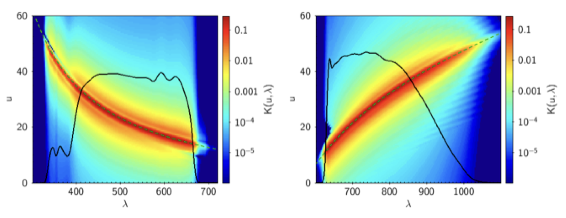
Figure 5.15: Final instrument model for BP (*left*) and RP (*right*) sampled on regular wavelength and pixel grids. Over-imposed black curves represent the instrument overall responses, while dashed green lines represent the dispersion functions.

The final instrument models for BP and RP are shown in Figure 5.15 where the corresponding instrument matrices sampled on regular wavelength and pixel grids are visualised together with the instrument response (black curves) and dispersion (dashed green curves).

Wavelength calibration accuracy

The accuracy of the wavelength calibration has been estimated by comparing the BP and RP mean spectra of a dataset of 102 QSOs with simulated spectra obtained by the convolution of the ground based spectra of these objects with the instrument model. The comparison, based on the wavelength position of 263 emission lines, shows that in general the accuracy is within 1%, except for $\lambda<$ 400 nm, where it is worse due to the scarceness of QSOs with emission lines in that range, and the presence of a systematic difference of 1 nm in RP, caused by the inability of the LSF model (see Section 5.3.5) to reproduce the instrument chromaticity. For more details, see Section 6.3 of Montegriffo et al. (2023).

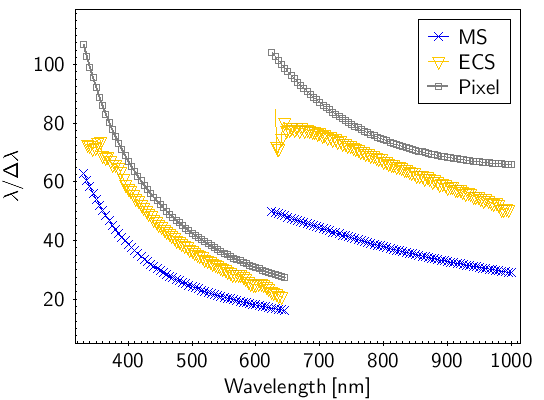
Resolution of calibrated spectra

The spectral resolution of the calibrated spectra is shown in Figure 5.16. An accurate description of the process to determine it can be found in Section 6.2 of Montegriffo et al. (2023), here we just report the findings: the variation of the resolution with the wavelength is more uniform in RP than in BP; below 650 nm there is a sudden decrease in the RP resolution of the externally calibrated spectra, while BP shows small oscillations around 600 nm, probably caused by ripples in the response profiles. The resolution of a typical Gaia externally calibrated spectrum falls from $R_{\lambda}=70$ to $R_{\lambda}\sim 22$ in the wavelength range $\lambda\in[330,640]$ nm, then jumps up to $R_{\lambda}\sim 78$ to decrease smoothly to $R_{\lambda}\sim 55$ at longer wavelengths.

Figure 5.16: Spectral resolution as function of wavelengths for BP and RP mean spectra (blue crosses) and externally calibrated spectra (yellow triangles), compared to the resolution corresponding to the width of one CCD pixel (grey squares).

Validation

The validation of the instrument models and the calibrated spectra was carried out by comparing the observed Gaia mean BP and RP spectra with the spectra obtained by feeding known SED to the instrument models. This comparison can be performed on sampled internally calibrated spectra (see Section 5.3.5) or on externally calibrated spectra (see Section 5.3.5). The dataset used for this purpose contains the SPSS and PVL sources (see Section 5.6 and Section 5.6.1) and the Next Generation Spectral Library (NGSL, Heap and Lindler (2016)), consisting of about 350 sources within the $G$ range [1.97–12.0].

Sampled mean spectra residuals

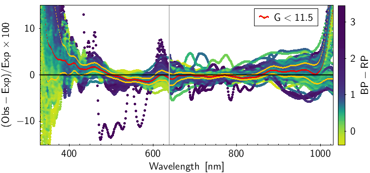
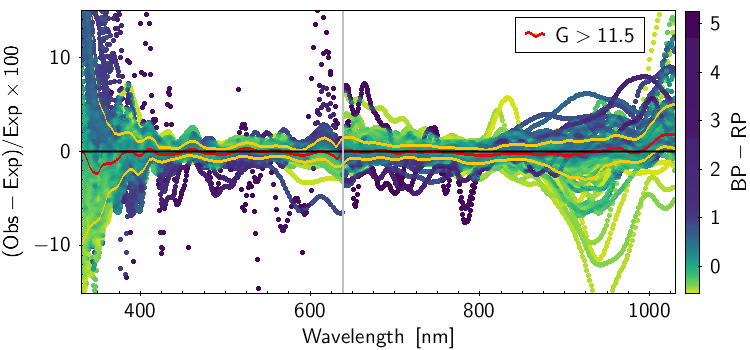
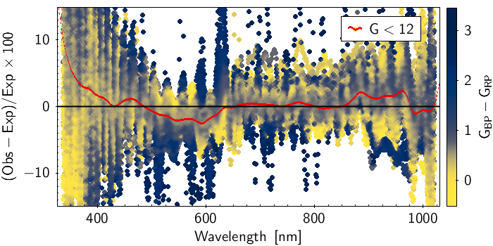
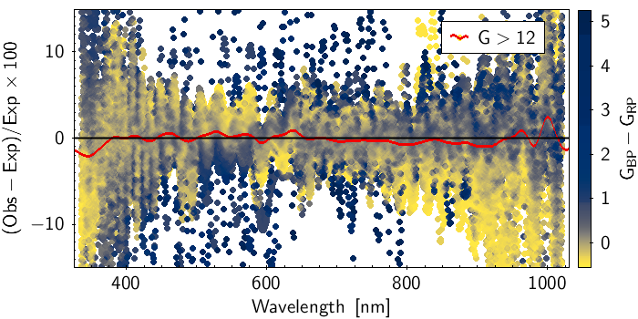
Figure 5.17 is an example of comparison between a mean and a simulated spectrum. This was carried out on the whole dataset and the residual, defined as percentage difference between the observed spectrum and the model prediction, was calculated. Figure 5.18 shows the residuals for the whole dataset, where each curve is colour-coded for the colour $G_{\mathrm{BP}}-G_{\mathrm{RP}}$ of the source. The grey vertical line marks the boundary between BP and RP wavelength ranges. The red and yellow curves represent the median and the $P_{16}$ and $P_{84}$ percentiles distributions. The two plots show different magnitude ranges as labeled in the figure, corresponding to the different window classes in the BP and RP spectra. The fact that the results are slightly different for the window classes implies that the internal calibration of bright sources did not converge fully to the mean reference system (see Section 5.3.4), mostly dominated by faint sources observed as 1D windows. For more details see Section 7.0 of Montegriffo et al. (2023)

Figure 5.17: Comparison between mean observed (in blue for BP, in red for RP) and predicted spectra (grey). The yellow curve represents the source SED rescaled in flux.

Figure 5.18: Percentage difference between observed and simulated mean flux for the validation dataset. See text for a detailed explanation.

Sampled calibrated SEDs residuals

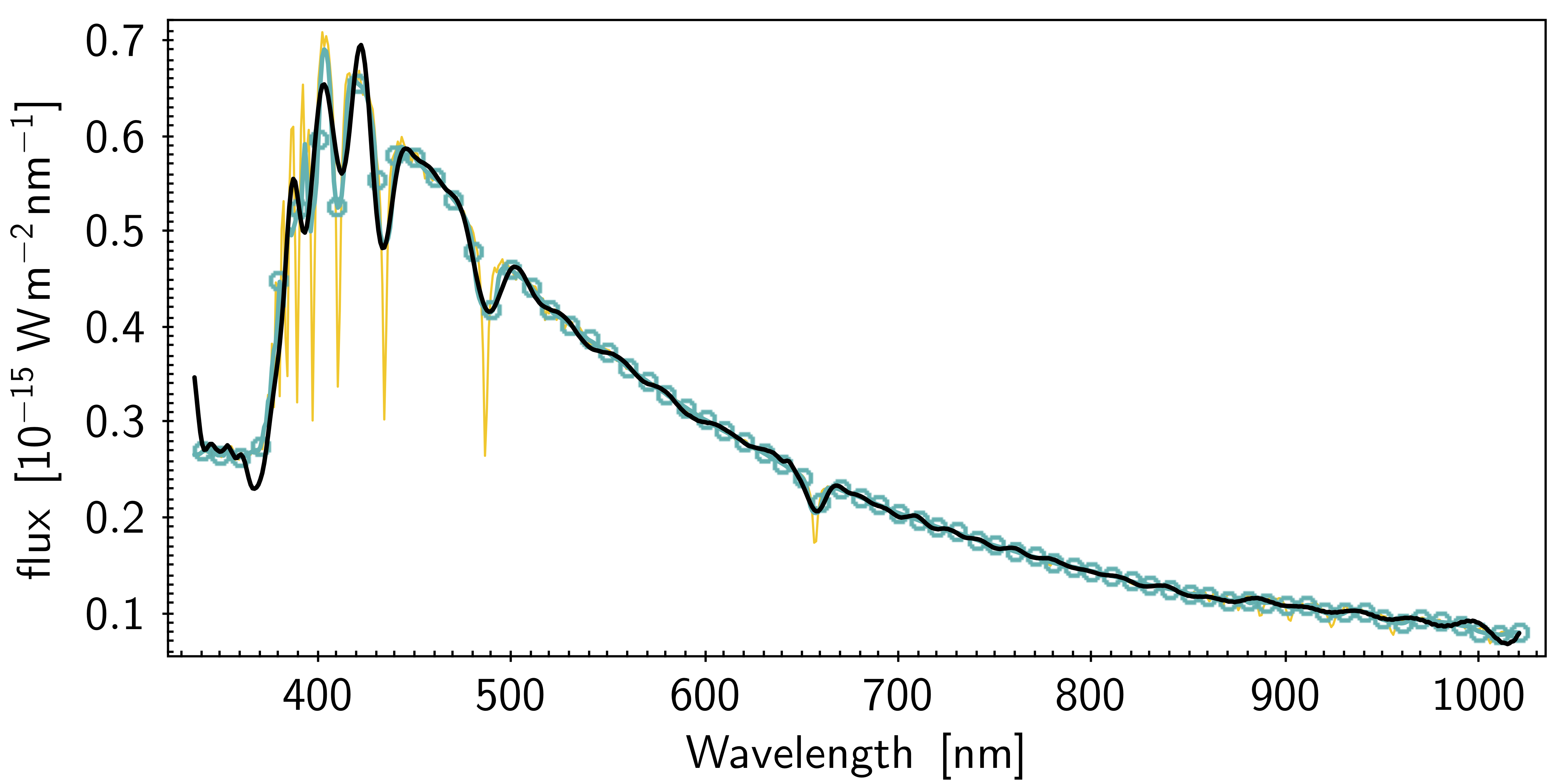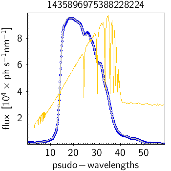
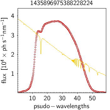
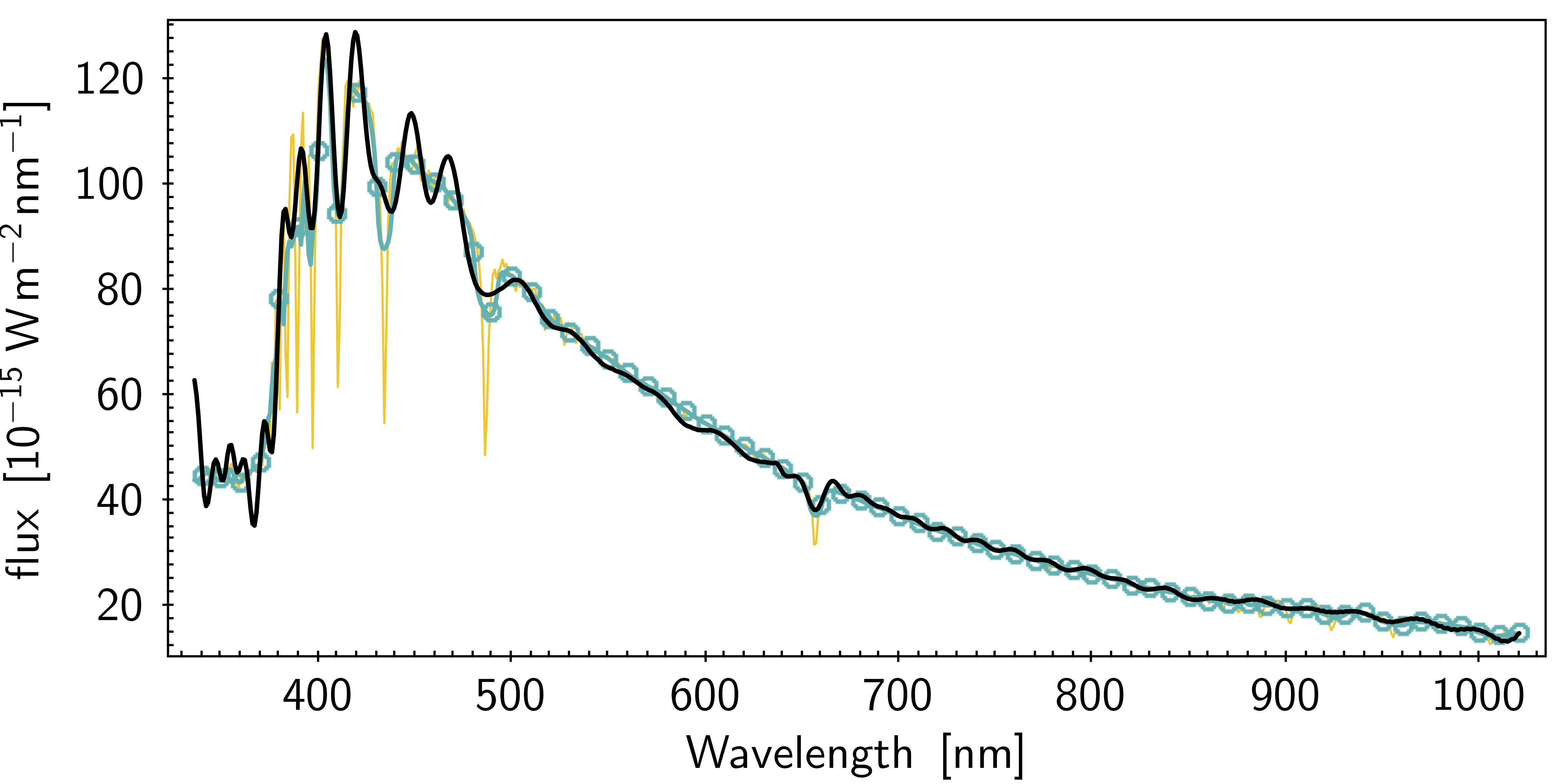
Figure 5.19: Comparison between externally calibrated (in black) and model SED (the yellow line represents the input high resolution external spectrum, the aquamarine circles represent the SED degraded to Gaia spectral resolution) for (from left to right) a bright and faint source respectively.

Figure 5.19 shows two example of comparison between a Gaia externally calibrated spectrum and the model SED obtained by applying the instrument model to the corresponding high resolution external spectrum of the same source: in both cases there is good agreement between the observed and simulated spectra, however the left spectrum exhibits wiggles. The presence of the wiggles is due to the basis inversion process (see Section 5.3.5) and their intensity can change significantly. Figure 5.20 shows the percentage residuals for the whole validation dataset, obtained comparing the externally calibrated spectra with the reference spectra, colour coded for the colour $G_{\mathrm{BP}}-G_{\mathrm{RP}}$ of the sources. While the wiggles are clearly visible, the median of the distribution (red line) behaves very similar to the corresponding median of the internally calibrated mean spectra (Figure 5.18).

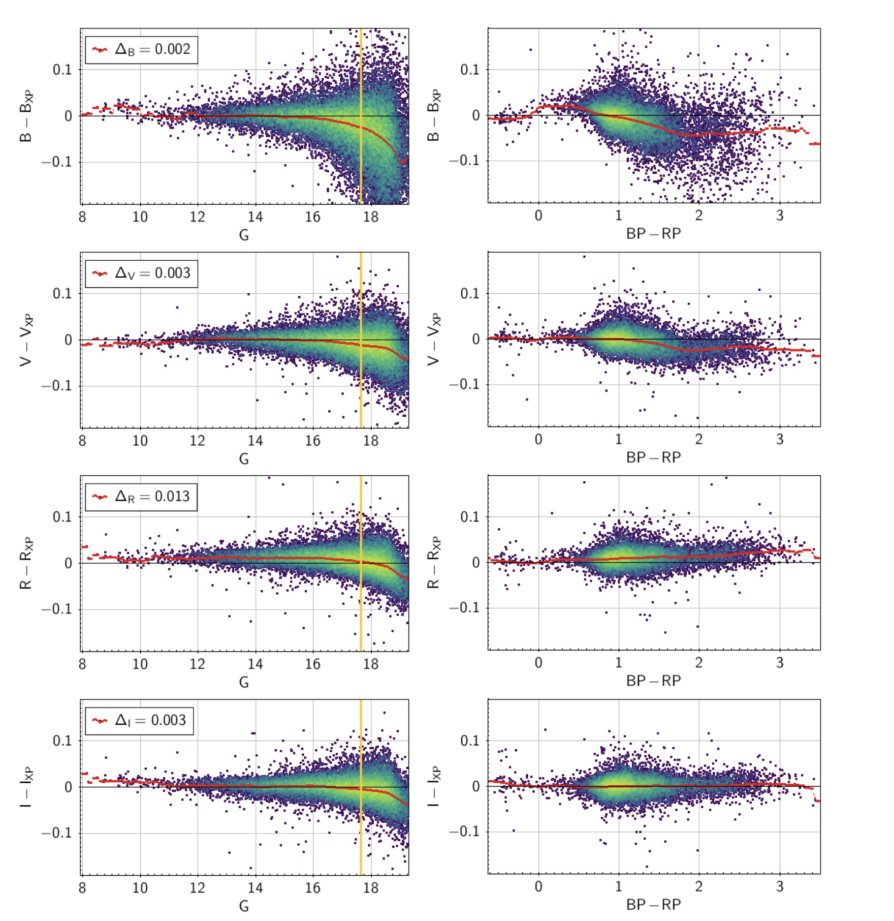
Figure 5.20: Percentage residuals between the externally calibrated fluxes and reference flux for the validation dataset. See text for a detailed explanation.

Comparison with external Johnson-Kron-Cousins photometry

The convolution of the calibrated Gaia low resolution spectra with filters in the wavelength range covered by the Gaia spectra allows to obtain wide and medium band synthetic photometry. The method and its validation is fully described in Gaia Collaboration et al. (2023g). An example is shown in Figure 5.21 where the BVRI magnitudes in the Johnson-Kron-Cousins system for a set of 32781 Landolt standard stars is compared with their synthetic BVRI photometry computed on externally calibrated BP and RP spectra. In the left panels of this figure is evident the presence of a magnitude dependent term for sources with $G$ $\geq$ 16, probably due to a systematic in the background estimation (see also De Angeli et al. (2023)).

gaia data release 3 documentation

5.3.5 External calibration

Instrument model

LSF model

Dispersion model

Response model

SED reconstruction

Processing

Results

Wavelength calibration accuracy

Resolution of calibrated spectra

Validation

Sampled mean spectra residuals

Sampled calibrated SEDs residuals

Comparison with external Johnson-Kron-Cousins photometry