7.6.6 Known issues
This is the first data release that includes EB orbital solutions and, as already mentioned earlier, there has only been a limited time to validate them or even properly address the problems that were discovered. One way to mitigate this situation was to limit the published sample to a small fraction of the original that satisfies a set of filtering criteria (cf. Section 7.6.5). However, even with this higher quality sample, there are a number of lingering issues and concerns of which the end user should be aware, and are discussed in this section.
Apparent inconsistency between and the overall quality of the fit
Perhaps the most obvious issue concerns the goodness-of-fit statistic, , which remains consistently high for most solutions (see Figure 7.53), thus giving the impression that most of them do not fit the data well. The reason for this is not entirely clear. should follow the normal distribution if the physical model applied is adequate, if the least-squares algorithm is capable of converging to the best fit, and if the estimates of the measurement uncertainties are right. There certainly are solutions where the fit is genuinely bad, most likely due to global optimisation failing to find a suitable reference LC. However, most such solutions have been filtered out by the process described in Section 7.6.5.
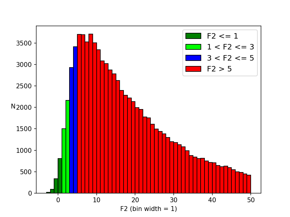
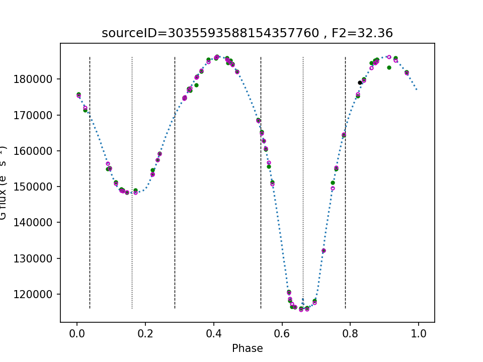
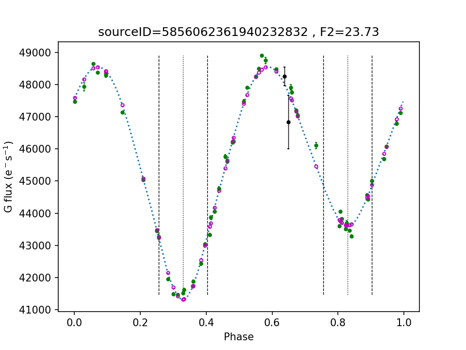
Figure 7.54 shows two examples of LCs for which the least-squares algorithm has converged to solutions that reproduce the bulk features of the LCs quite well, yet exhibit a large . Therefore, this must be due to inadequacies of the physical model, underestimated measurement uncertainties, or a mix of both. Shortcomings of the physical model may include ignoring intrinsic variability of the components or ignoring the presence of spots or circumstellar disks, but may also be related to an inferior numerical accuracy of the simulator output compared to the accuracy of Gaia photometry. At the same time, underestimated measurement uncertainties cannot be discounted as the calibration effort of Gaia photometry is still ongoing. These scenarios, along with possible remedies (such as adding jitter to the model fluxes when appropriate) are currently under investigation.
In the meantime, and as a way of facilitating filtering operations performed on the basis of the goodness of fit (such as in Section 7.6.5), the g_rank, presented in Section 7.6.5, offers the possibility of ranking LCs based solely on the flux values of their data points, unaffected by concerns about their uncertainties.
Reliability of parameter uncertainties
The quoted uncertainties for the fitted parameters come from the covariance matrix of the solution, as calculated by the Levenberg-Marquardt method. However, the off-diagonal elements of the covariance matrix are a measure of the pairwise correlations between parameters to first order only. More realistic uncertainties may be provided by MCMC simulations, but these were out of scope for Gaia DR3. This implies that the reported parameter uncertainties are likely generally underestimated. It should also be reminded that the calculation of the covariance matrix involves the computation of numerical derivatives which are sometimes of limited accuracy.
Uncertainty for actually refers to
The time reference calculated by the local optimisation is , the time when the primary component is eclipsed by the secondary. However, as mentioned in Section 7.6.5, the published time reference is instead , the time of periastron passage. However, the transformation from to was done only for the value of the parameter, and not for its uncertainty. In other words, the provided uncertainty still corresponds to that of . This oversight was discovered too late to be corrected for Gaia DR3.
Error in the calculation of mutual irradiation effects
Late in the validation process, it was discovered that a software bug in the mutual irradiation algorithm (cf. Section 7.6.3) disables the calculation of irradiation effects under certain conditions. This bug is expected to mostly affect solutions for systems characterised by a combination of large fill factors and a significant temperature difference.
Spurious non-circular systems for arguments of periastron close to and
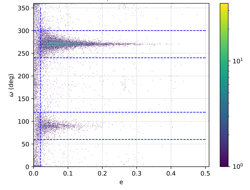
When an EB is viewed along its semimajor axis, i.e., when or , it is not possible to determine from its LC whether it is circular or eccentric, especially in the case of a detached system. This is an inherent degeneracy of the problem that occurs because even if the system is eccentric, the eclipses still occur half a period apart. During local optimisation, nothing prevents the Levenberg-Marquardt algorithm from fitting a near-circular system with an eccentric system having an argument of periastron close to or . This effect causes an excess of spurious eccentric solutions around these angles, as shown in Figure 7.55. In order to reduce the number of these spurious solutions, they were filtered out when and . However, it should be expected that a number of non-excluded solutions with around the affected regions are also, in reality, circular orbits. Although this degeneracy cannot be fully avoided, future data releases can attempt to mitigate it, for example by trying circular solutions near these angles, and by improving the performance of global optimisation.
Inclination angles exceeding 90
It is not possible to detect retrograde motion from EB LCs. Therefore, there is no meaning in reporting inclination values exceeding . However, in order to avoid having the interesting case of mapped near the edge of the logit transformation that is used to constrain the local optimisation, was left to vary up to . Unfortunately, by omission, its value was not mapped back to , so it is incumbent on the end user to perform this transformation.
Third light ignored
When a “third” source of light, usually a background or foreground star, is included in the photometry of an EB, it has the effect of rendering the eclipses more shallow, roughly emulating a system with a lower inclination. This effect should be more common with fainter EBs located in dense stellar fields. Although the EB simulator has the ability of fitting a third light, it was not enabled because it cannot be done robustly with a single-passband LC.
The period is not fitted
The period of photometric variability, and hence also the orbital period of the EB, is taken from variability processing, as mentioned in Section 7.6.2. Preliminary experiments to include the period as a free parameter in model fitting did not bring any improvement, at least in the context of the split global-local optimisation scheme currently employed. This also means that the uncertainty in the period is not taken into account when computing the covariance matrix of the solution (i.e., its influence on the uncertainties of other parameters is ignored).