6.1.2 Overview of the spectroscopic processing
The spectroscopic processing pipeline is the result of the work of the CU6 (Section 1.2.2): the scientific teams provide the scientific codes to DPCC (CNES), who integrates them in the SAGA (System of Accommodation of Gaia Algorithms) host framework. SAGA is developed by Thales. The pipeline is run at DPCC on an Hadoop cluster with 1100 cores. The processing took approximately 630 000 hours CPU time and needed 290 TB disk space. The auxiliary data are produced off-line by the scientific teams.
The purpose of this first version of the spectroscopic pipeline is to estimate the radial velocity of the brightest stars observed by the RVS. The basic functionalities, sufficient to treat the brightest stars with non-truncated windows, have been implemented. No deblending of the spectra of overlapped sources’ spectra is attempted (the spectra having truncated windows are simply excluded from the data flow, and the contamination of the sources not observed by the RVS with their own window is neglected). The calibration of the spectra is limited to the wavelength calibration (indispensable for the radial velocity estimation) and to the electronic bias non-uniformity mitigation (the non-mitigated spectra present jumps that perturb the radial velocity estimation). The along-scan Line Spread Function (LSF-AL) calibration has been done off-line and two models have been produced: the first one was obtained using the RVS data of the first month of the mission, when the RVS resolution was degraded by water ice optics contamination, and was used for the data acquired before the decontamination at OBMT 1317 (Figure 6.1); the second one, obtained using on-ground data, was used afterwards, when the resolution returned to nominal values. Similarly, the nominal instrument response has been used. The across-scan Line Spread Function (LSF-AC) calibration was not required because the possibility of deblending windows was switched off. The straylight calibration has been done off-line and no temporal variations are considered. The calibration models used are described in Section 6.3. All the missing functionalities will be implemented in later pipeline versions, when fainter stars will be treated.
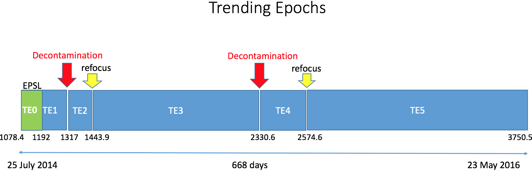
Trending Epochs: The study on the wavelength calibration temporal evolution has shown that the decontamination and the refocusing events produce discontinuities in the wavelength calibration zero point. In the Gaia DR2 dataset, which includes the data acquired between 25 July 2014 (OBMT 1078.4) and 23 May 2016 (OBMT 3750.5), there are two decontamination events, each followed by a refocusing event. In addition, also the EPSL/NSL transition (OBMT 1192.1) produced a (smaller) discontinuity. These five events have been defined as breakpoints and the dataset has been separated into the six trending epochs shown in Figure 6.1. For each trending epoch a wavelength calibration model is estimated.
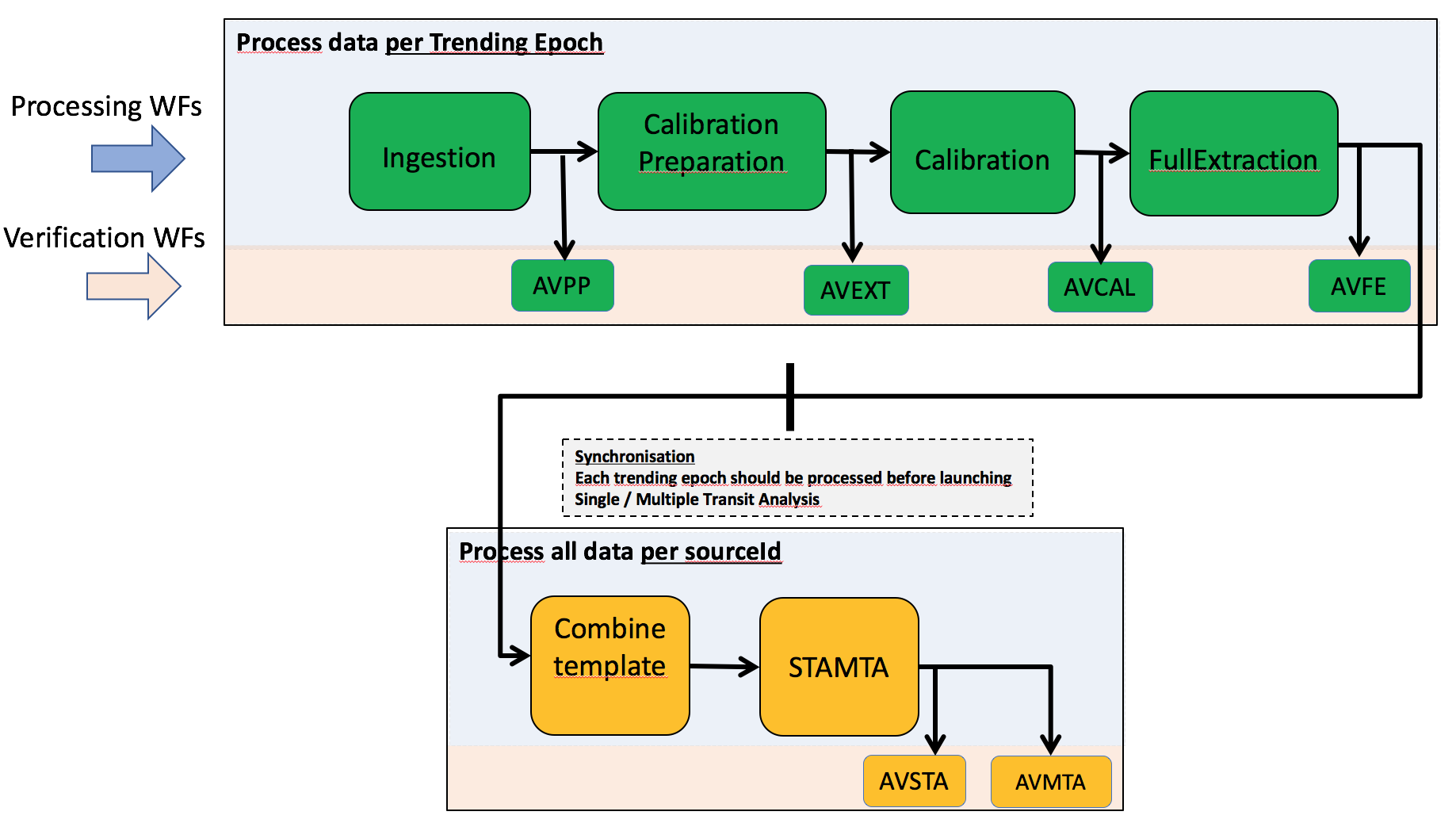
In Figure 6.2 the pipeline processing steps, technically called workflows, are represented. There are six processing workflows that are followed by Automated Verification (AV) workflows. The AV workflows are in charge of verifying the products obtained by the processing workflows. Each workflow coloured in green in the figure processes the pertinent data of an entire Trending Epoch, and has to be finished before the following workflow starts. The data are processed per-transit or, in the Calibration workflow, per calibration unit (i.e. a dataset covering 30 hours of observation containing the calibration stars and the standard stars). The last two steps (coloured in yellow) are integrated after a synchronisation process, where the data produced in the previous workflows for all the transits relative to each source are grouped. The processing in the last two steps can start only when all the preceding workflows for all trending epochs are finished, and the data products for all transits are produced. The objectives and main products of each processing workflow are described in Section 6.4. The objectives of the AV workflows are described in Section 6.5.1.