5.4.2 BP/RP processing

In the current release only the most dominant contribution to the background is calibrated and then subtracted, that is the one from the stray light. For this, the models described in Section 5.3.1 are used. If in the maps there are empty bins, interpolation between the neighbours is performed to fill them. The completed map is then used to build a bicubic spline interpolator which, given the heliotropic spin phase and the AC coordinate of the transit to be corrected, computes the background value in electron/pixel/second. This value is converted to the appropriate one, depending on the window sampling (1D or 2D), and then subtracted to the transit to be corrected.

As the calibration for the charge release is not yet available, only the transits with a distance from the charge injection bigger than 50 TDI are processed at this stage.

The differential dispersion function and geometric calibrations are carried out simultaneously. The differential AL geometric and dispersion calibration is determined with respect to an initial fixed arbitrary reference sample position (ARS), and using observations of a sub-sample of the sources selected in a narrow range of colour to ensure that they are of similar spectral types (and their spectra are therefore quite similar).

The calibration proceeds through the following steps:

• •

  Alignment

  • –

    Initial estimate of the set of AL position shifts and flux scaling factors to be applied to the observed spectra in a given calibration unit to align them with each other. All the suitable observed spectra are first normalized to a given magnitude (set in the configuration). Within each calibration unit then, all spectra are cross-correlated using a spectrum that is observed at AC position close to the CCD centre (and therefore is representative of an average dispersion) as reference. The result of this process is a set of AL position shifts and scaling factors, one per input spectrum.

  • –

    Refinement of the set of shifts and scaling factors found in the previous step. This is achieved by fitting a spline to all the observed spectra (after applying the adjustments found in the previous step) in one calibration unit. There will be one spline (reference spectrum) per calibration unit. A correction to the shift and scaling factor first estimates is computed by fitting each of the observed spectra back to the corresponding reference spectrum spline. This is an iterative process where at each iteration a new reference spectrum is computed. The result of this process is a new set of shifts and scaling factors.

• •

  Differential dispersion calibration In this step the algorithm runs on a set of binned spectra (one per calibration unit) defined using the adjusted spectra obtained from the previous step. Each binned spectrum is computed on a fixed grid, the value of the binned spectrum at each bin is computed as the weighted mean of all observed samples (from all available transits) falling within the bin range. The binned spectra are thus compared to compute a set of additional AL position shifts (one per calibration unit) and a set of corrections for the nominal differential dispersion functions (again one per calibration unit). This is achieved in an iterative process where each iteration consists of two steps:

  • –

    a spline is fitted to all the input binned spectra by iteratively adjusting the set of AL position shifts and scaling factors (one per calibration unit);

  • –

    an LSQ fit is done with all the input binned spectra and the fitted spline to obtain as a result a set of AL position shifts and corrections for the nominal differential dispersion functions (one per calibration unit).

• •

  Differential geometric calibration The differential AL geometric calibration is finally derived as the median of the difference between the location of an arbitrary reference sample (ARS) in the observed spectrum (given by the ARS location in the reference system adjusted by all the shifts computed so far, the AL position shift per epoch spectrum computed in the alignment and the additional shift per calibration unit computed in the differential dispersion calibration) and the predicted AL data space coordinate for each transit.

  It is probably necessary to spend a few more words on the definition of the arbitrary reference sample (ARS). This is the AL location of an arbitrary effective wavelength. For the internal calibration it is irrelevant to know what this wavelength is. The differential AL geometric calibration is defined with respect to the location of the ARS. The application of the geometric calibration determines the observed location of the ARS expressed in pixels within the window.

  In future cycles, the location of the ARS will be optimized to make sure that the difference between effective wavelength and nominal wavelength is at its minimum in the vicinity of the ARS for different spectral types. Each sample position corresponds to a given nominal wavelength through the dispersion function. However in general this wavelength is different from the effective wavelength (which is the average wavelength weighted by the spectrum shape and therefore clearly depends on the spectral type). In order to make sure that the chosen ARS is consistent over a large range of spectral types, one needs to select a sample position where the difference between the nominal and effective wavelength has a minimum.

  For Cycle 02, no optimization was done and the nominal values for reference sample and corresponding wavelength were adopted.

The application is done on all observed spectra. It consists of two steps:

• •

  Differential geometric calibration application: defines for each observed spectrum the AL location of the reference effective wavelength. This is referred to as the observed ARS.

• •

  Differential dispersion calibration application: converts the observed sample AL positions into the pseudo-wavelength system. As mentioned, only nominal dispersion functions were used for Cycle 02 processing (and for the generation of the data included in Gaia DR2).

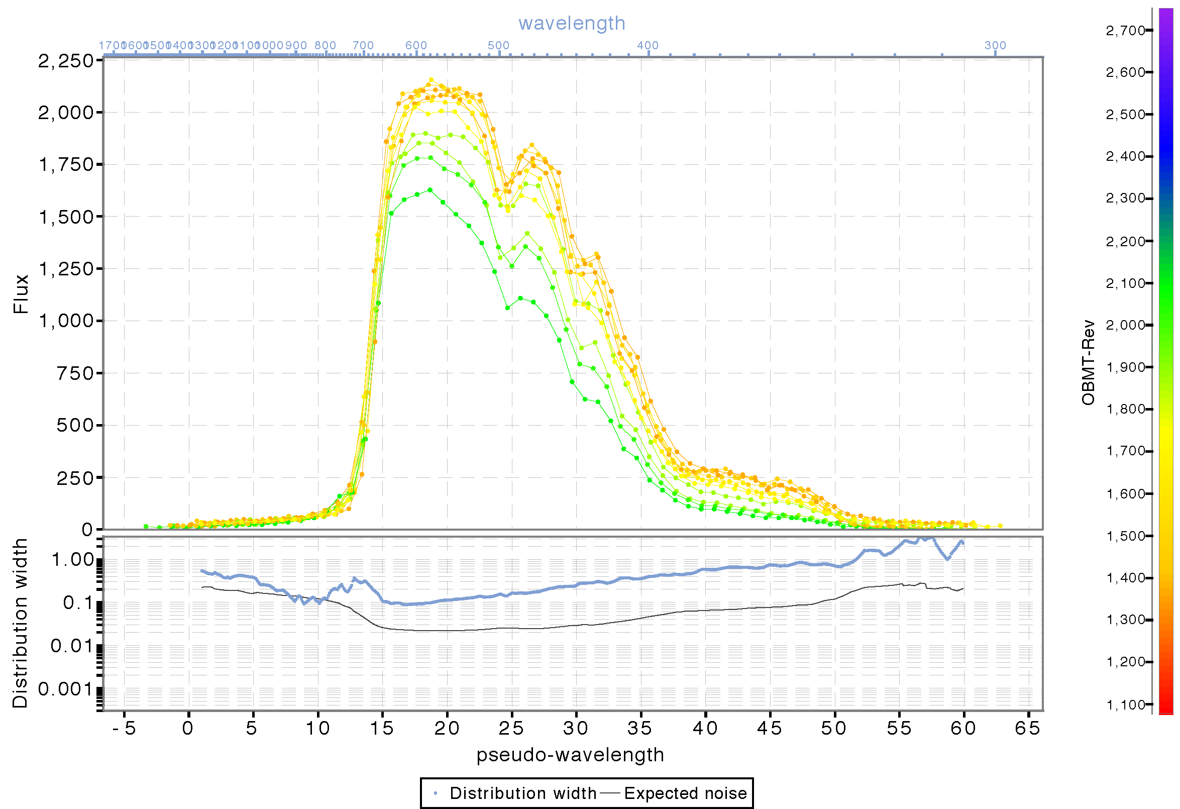
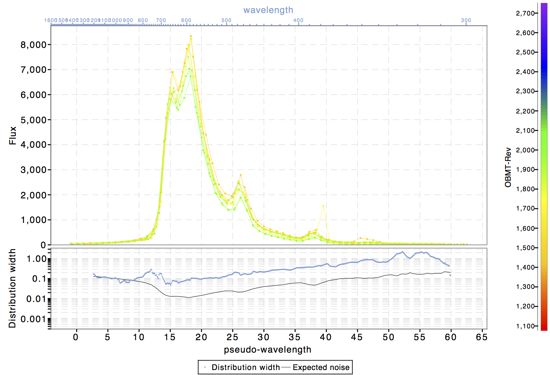
Figure 5.23 and Figure 5.24 show two examples of epoch (BP) spectra. Figure 5.23 is for an SPSS source while Figure 5.24 is for an emission line source. Here all epoch spectra have been calibrated for background, differential dispersion and geometry achieving a good alignment of the main features. Clearly no flux and LSF calibration has been applied, and contamination effects (varying with time) are quite evident and still present in the spectra. These will be taken care of in future cycles.

For Gaia DR2, SSCs were computed on epoch spectra calibrated for background, differential dispersion and geometry assuming nominal absolute dispersion. These SSCs then get calibrated within the photometric processing.