11.3 Apsis modules 11.3.11 Total Galactic Extinction Maps 11.3.13 Unresolved Galaxy Classifier (UGC)

11.3.12 Outlier Analysis (OA)

Author(s): Daniel Garabato, Minia Manteiga, Lara Pallas-Quintela, Marco A. Álvarez, Carlos Dafonte

Goal

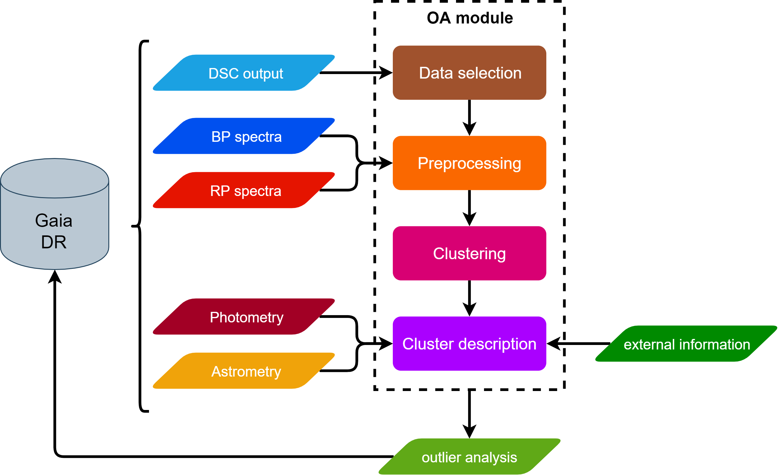
OA aims to complement the overall classification performed by the DSC module by processing those objects with a lower probability classification from DSC (see Section 11.3.2). It aims to help in the photometric processing by detecting artefacts, improving DSC classification and analysing weird, infrequent objects. Specifically, it deals with the analysis of those sources that are assigned DSC combined probabilities below a given threshold for all the considered classes (see Delchambre et al. 2023). Figure 11.50 shows the OA processing stages, which are briefly described below.

Figure 11.50: Flowchart diagram of the Outlier Analysis (OA) module.

In order to select an object as an outlier, we require that all its DSC combined probabilities (associated with each DSC class) stand below a given threshold, $\theta<0.999$ . The main goal of OA is to extract knowledge from these sources, so that the underlying cause of their classification as outliers can be identified and understood. In order to analyse them, OA performs an unsupervised classification (clustering) by means of Self-Organizing Maps (hereafter SOM, Kohonen 2001; Ordóñez et al. 2012; Fustes et al. 2013; Dafonte et al. 2018), grouping similar objects according to their BP/RP spectra. In addition, OA characterises each group of similar objects, i.e. cluster or neuron, by reporting statistics of the main Gaia computed quantities: magnitudes, galactic latitudes, parallaxes, number of transits, etc. The quality of the clustering is also assessed according to different measurements on the distribution of classification distances, so that a quality category can be identified for the neurons, as detailed in Section 11.3.12.

Finally, a class label is assigned to the best clusters following a template matching procedure detailed in Section 11.3.12. It must be noticed that we characterise and label clusters instead of objects. Since a cluster is representative of the sources that are assigned to it, those properties could also be extrapolated to the sources it contains. A classification distance, as well as a distance percentile, are defined for each source, so that the final user can decide whether to make such properties extensive or not for a particular source.

Inputs

OA internally uses mean XP spectra produced by SMSgen (Section 11.3.1), downsampled to 60 pixels, concatenated (as it is shown in Figure 11.51), and preprocessed before the clustering is performed in order to deal with border effects, zero or negative pixels, as well as the overlapping region between BP and RP wavelengths (see Section 11.3.12). Additionally, some internal Gaia information, such as sky coordinates (b), magnitudes in Gaia bands (phot_g_mean_mag, phot_bp_mean_mag, and phot_rp_mean_mag) or the number of transits (phot_bp_n_obs, and phot_rp_n_obs) are used to describe the objects grouped in the same neuron.

Method

The method used by OA to analyse the nature of classification outliers is an unsupervised Artificial Intelligence algorithm, namely Self-Organized Maps (Kohonen 2001) which allows to group objects with similar spectral energy distributions and does not make use of any prior knowledge based on physical models. Some optimizations were introduced to speed up the execution of the module, and different validation mechanisms were also implemented.

Preprocessing

Many of the spectra processed by OA come from low apparent luminosity objects, which as a result of the extraction process can have pixel intervals with very low or even negative fluxes. To carry out a meaningful clustering for as many objects as possible, a preprocessing stage is performed before training the SOM model.

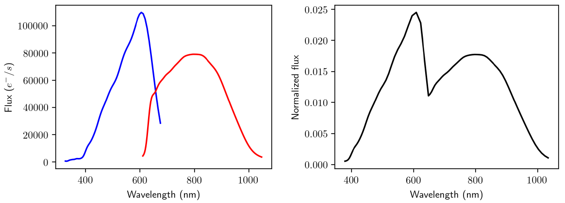
This procedure is illustrated in Figure 11.51 and allows to improve the overall performance of the model. It consists of the following steps:

1.

The borders of each spectra are trimmed due to the low transmission at these wavelengths. As a result, OA uses the effective wavelength ranges $[375,644]$ nm for BP and $[644,1050]$ nm for RP.
2.
Some spectra may contain negative flux values, and therefore such regions are linearly interpolated provided that they comply with the following constrains:
- –
  
  A maximum of 10% of the effective wavelength range is allowed to present consecutive negative flux values.
- –
  
  A maximum of 25% of the effective wavelength range is allowed to present negative flux values spread all over the spectrum.
Otherwise, the sample is considered to be a poor quality spectrum and it is discarded.
3.

After some experimentation with XP spectra at different spectral resolution, we decided to downsample the spectra from 120 to 60 pixels, as the quality of the clustering does not change substantially. This allowed to reduce the execution times without losing performance.
4.

Both BP/RP spectra are joint in a single array of fluxes, whose wavelengths are sorted in strictly ascendant order.
5.

Finally, the resulting spectrum is normalised, so that its area sums up to one.

Training

Self-Organizing Maps are a non-supervised technique based on neural networks. These maps perform a projection of a multidimensional input space in a two-dimensional grid, facilitating its visual exploration using the appropriate tools. This projection is characterised by preserving topological order; that is, similar data in the input space will belong to the same neuron or to neighbouring neurons in the output space. Each one of these neurons has a representative, called a prototype, which is a virtual pattern that is adjusted during the training phase and that best represents the input patterns that belong to such a group. Beware that the membership of a source to a neuron is determined by identifying the closest neuron prototype to the given source.

Due to the large amount of data to be processed in the current context, we optimised the base SOM algorithm by using the so called Fast-SOM version (Dafonte et al. 2018), which was designed and implemented for distributed computing environments. One of the most important processing steps involves the calculation of the neuron prototype. In the case of the SOM computed for Gaia DR3 outliers, each neuron prototype was calculated as the average spectrum for all the XP spectra of the sources contained in that particular neuron. Such a simple representation was achieved because of the configuration used and the execution performed, where the number of iterations was large enough to reach a neighbourhood radius (which represents the topological distance between neurons) equal to zero (Kohonen 2001) during the computation of this specific SOM map.

In order to set-up the SOM for Gaia DR3, the following variables were appropriately tuned and configured according to the results obtained during an extensive experimentation phase:

•

Grid of neurons: $30\times 30$ (900 neurons).
•

Similarity function: squared Euclidean distance.
•

Neighbourhood function: Gaussian.
•

Maximum number of iterations: 250.
•

Activation of the Fast-SOM mode: 20% of iterations (50 in this case).

Clustering quality assessment

When it is not possible to resort to any a priori information about the physical nature of the objects that populate the neurons, since such nature is unknown, clustering quality assessment based on classification success rates cannot be performed. In this case, internal parameters can be used to measure the quality of the grouping and to validate the SOM algorithm performance. We have chosen to carry out a descriptive approach to analyse the quality of the grouping, based on inter-neuron and intra-neuron distances (Álvarez et al. 2021).

On the one hand, the inter-neuron distance is computed as the squared Euclidean distance between two different neuron prototypes. For each neuron, some statistical values are calculated just taking into account its immediate neighbourhood. On the other hand, the intra-neuron distance is computed as the squared Euclidean distance between a source and the prototype of the neuron where it belongs, so that different statistics can be calculated on the sources populating each one of the neurons.

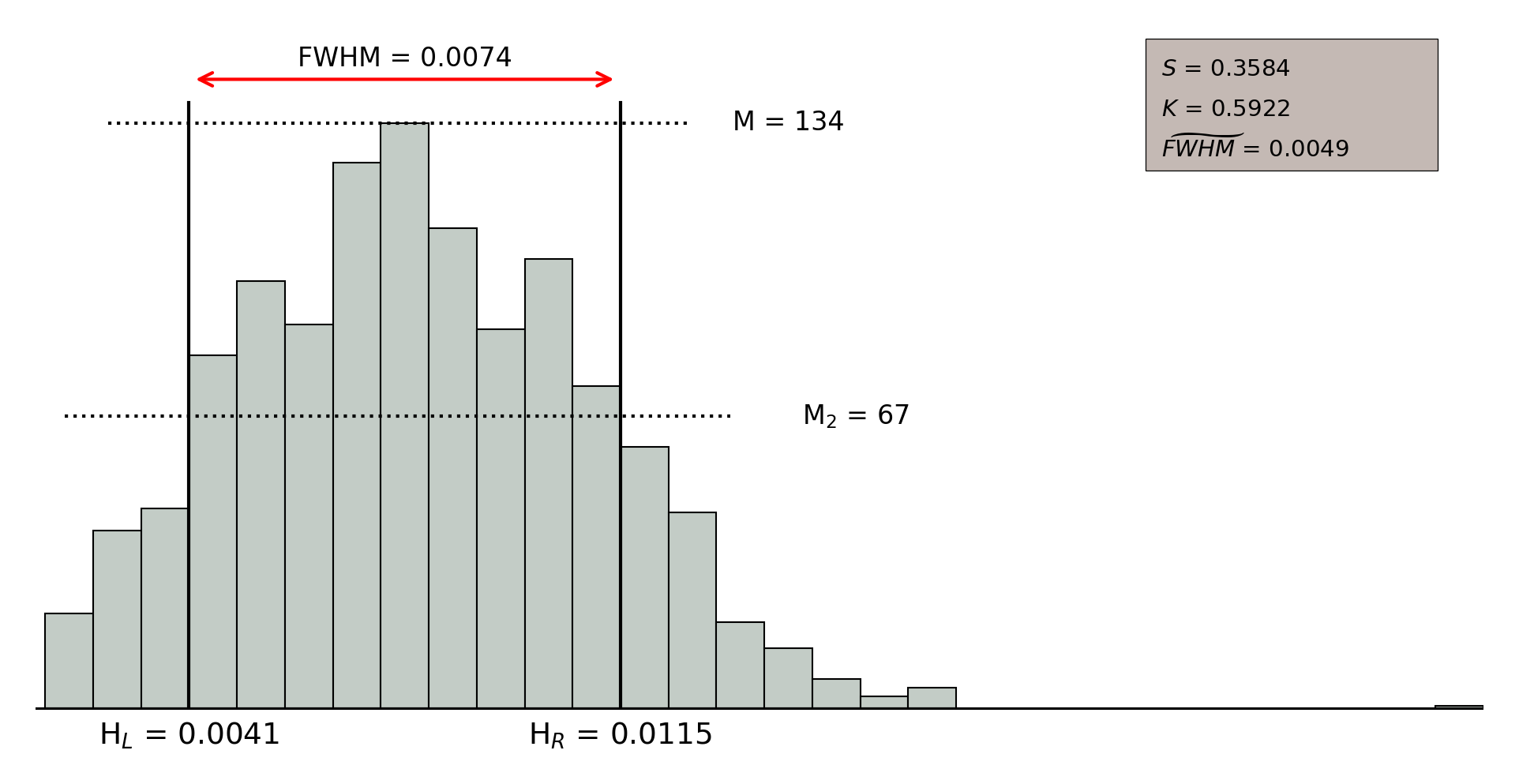
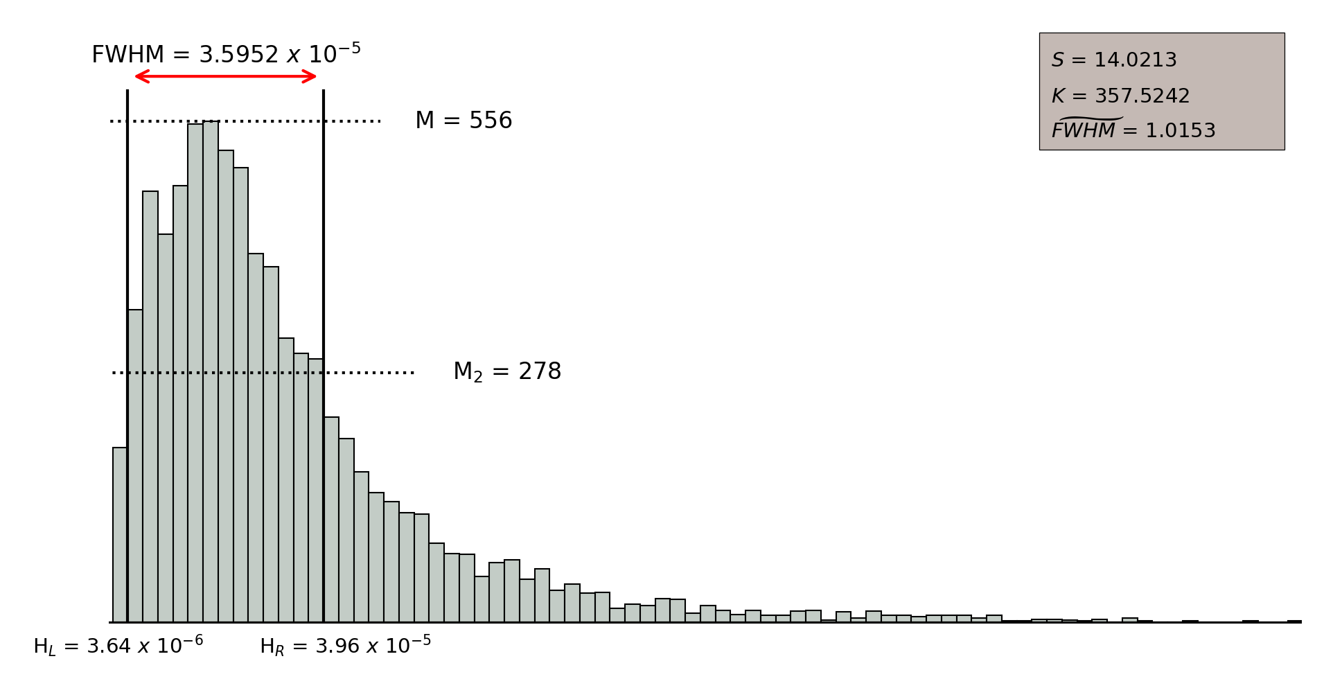
In order to assess the quality of the clustering, we selected three parameters that allow to describe the distribution of the intra-neuron distance: a) the width of the distribution according to the value of the $F W H M$ (Full Width at Half Maximum); b) the skewness ( $S$ ) that measures the asymmetry of the distances distribution; and, c) the kurtosis ( $K$ ), that measures the level of concentration of distances. A high quality clustering will result from neurons with low values of the $F W H M$ parameter, and large positive values of both skewness and kurtosis.

Additionally, a fourth quality parameter was defined to quantify the quality of each neuron with respect to the other ones, so that they can be easily compared. Therefore, $\widetilde{FWHM}$ was introduced as a scaled version of $F W H M$ , in which the average value of the $10\%$ of neurons with lowest $F W H M$ (that is, the best ones) is used as the scale factor. Finally, in order to facilitate the interpretation of quality measurement, we have derived a new categorical index named $Q C$ , which is based on the values obtained for the three parameters discussed above: $\widetilde{FWHM}$ , $S$ , and $K$ . Seven quality categories were empirically established to rank $Q C$ according to the values of such parameters in six percentiles ( $95^{th}$ , $90^{th}$ , $75^{th}$ , $50^{th}$ , $32^{nd}$ , and $10^{th}$ ), defined independently for each parameter distribution. For each neuron, we determine the lowest percentile in which the three parameters are above their respective percentile values. Thus, if such value is in the 95 ${}^{th}$ percentile, then $Q C$ will take value zero; if it is in the $90^{th}$ percentile, then $Q C$ will correspond to category one, and so on up to category six, which will correspond to those neurons whose worst quality indicator is outside the lowest percentile that has been considered, $10^{th}$ . Accordingly, the best quality neurons will have $QC=0$ and the worst ones; $QC=6$ .

Figure 11.52 shows an example of intra-neuron distance distributions for those objects populating two different neurons. On the one hand, the upper figure illustrates a low quality neuron, which takes small values for $S$ and $K$ , so that the distribution looks more symmetric and the distance values are spread all over the distribution rather than concentrated in a specific range, which is also supported by the large values taken by the $F W H M$ . On the other hand, the lower figure shows the intra-neuron distance distribution for a high quality neuron, where parameters $S$ and $K$ take large values and $F W H M$ takes a small value, meaning that the distance distribution is clearly skewed to the left and it concentrates a large amount of sources classified with small distance values.

Figure 11.52: Example of quality measurements for two different neurons: a low quality neuron (LQN, upper panel) and a high quality neuron (HQN, lower panel). The intra-neuron distance distribution is shown where M is the peak value and M ${}_{2}$ if the half of the peak value. H ${}_{L}$ is lowest value at half maximum, while H ${}_{R}$ is the largest value at half maximum.

Template matching

Self-Organised Maps (SOM) are a powerful Data Mining tool to extract knowledge from complex and multi-dimensional data, such as Gaia data. However, due to their unsupervised nature, these maps do not provide any type of label that can be associated with the samples that are being analysed. For this reason, a template matching procedure was included as part of the neuron description phase, so that a class label can be determined for each one of the neurons by using a set of reference templates. In this way, such templates help to study the physical nature of those outlier sources that populate a certain neuron in the OA SOM map.

For this purpose, a wide variety of objects with reliable classification in other astronomical catalogues was gathered, so that the most astronomical types expected in Gaia survey were appropriately covered. It is also worth mentioning that this reference catalogue was internally used for validation purposes of the SOM technique in order to assess their performance on Gaia data by means of common external evaluation metrics, such as precision, recall or F ${}_{1}$ -score. In order to build the templates, a SOM map was trained outside Apsis, and then the predominant label was computed for each neuron. Those neurons that achieved a qualified majority above 68% were selected as template candidates. Then, for each one of these neurons, the 68% of the closest sources to the prototype were selected, and their XP spectra was averaged to build the actual templates, which were associated with the corresponding predominant object type.

Such templates have been created with two levels of detail regarding the class labels, a basic label and a more specific one. On the one hand, the basic labels refer to broad spectral types for stars (early, intermediate and late), and extragalactic object types in wide redshift ranges. On the other hand, the specific set of labels considers finer levels of classification for both stars and extragalactic objects. All these label types that were considered can be observed in Table 11.32. In order to build the reference templates, a specific label is always preferred as it provides more information than a basic one. For this reason, we first tried to find predominant types by labelling the SOM map using specific labels. However, for those neurons that a specific label could not meet the qualified majority criteria defined above, we tried to apply basic labels to meet the criteria. Through this process, we were able to build 561 templates that represent specific labels (a single type may be represented by multiple templates), and 122 templates that are associated with basic labels.

Table 11.32: Class labels types used to build OA templates. For quasar and galaxy object types, the specified redshift range of the templates must be read as follows: Zab_xy should be translated to

z\in[a.b,x.y)

, while Zab_GT corresponds to

z\in[a.b,\infty)

, and Zab_LT should be interpreted as

z\in(\infty,a.b)

Type	Basic label	Specific label
Star	Star Early	Star O
		Star B
		Star A
	Star Intermediate	Star F
		Star G
	Star Late	Star K
		Star M
	White Dwarf
	Emission Line Star
	Carbon Star
	Physical Binary
Quasar	Quasar Z25_GT	Quasar Z45_GT
		Quasar Z35_45
		Quasar Z25_35
	Quasar Z15_25
	Quasar Z15_LT	Quasar Z05_15
		Quasar Z05_LT
Galaxy	Galaxy Z02_GT	Galaxy Z025_GT
		Galaxy Z02_025
	Galaxy Z01_02	Galaxy Z015_02
		Galaxy Z01_015
	Galaxy Z01_LT	Galaxy Z005_01
		Galaxy Z005_LT

These reference templates were used to label the neurons in the DR3 outliers SOM map by means of the k-NN method and the squared Euclidean distance, so that for each neuron the closest template to its prototype was identified. In addition, to guarantee the suitability of the assigned templates (and class labels), two conditions were imposed: a) the distance between a template and its prototype must not exceed a threshold $\Phi\leq 3.58\times 10^{-2}$ ; b) the neuron must be over a quality threshold based on the aforementioned indicators, where the categorical index $Q C$ must meet the condition $QC<6$ . Both criteria depend, at the same time, on the quality of the spectrophotometry, and the threshold values defined above were empirically determined based on the experimentation performed during the internal validation cycles in Apsis.

Therefore, those neurons that do not meet any of such conditions were not associated with a template and, hence, they were not assigned any class label either. Finally, it should be noted that the prototypes of neurons are synthetic and, therefore, they do not correspond to any real observation, but rather to the average XP spectra of the observations that populate the neuron. Note that the templates are also synthetic, based on the averaged XP spectra of several sources. For this reason, we also provide a centroid for each neuron, which represents the closest real observation to the neuron prototype, and it was determined, once again, by means of the squared Euclidean distance.

Outputs

OA contributes to the archive by means of different products:

•

Self-Organized Map (SOM) clustering for outlier sources using a $30\times 30$ map (900 neurons).
•

Neuron-by-neuron statistical description for different Gaia observables, such as $G$ , $G_{\rm BP}$ , $G_{\rm RP}$ , $\varpi$ or $G_{\mathrm{BP}}-G_{\mathrm{RP}}$ .
•

Neuron-by-neuron quality measurements, which comprise basic statistics on intra-neuron and inter-neuron distances, and some parameters computed for the intra-neuron distance distribution: Full Width at Half Maximum ( $F W H M$ ), skewness ( $S$ ), kurtosis ( $K$ ). Additionally, from these parameters a categorical quality index ( $Q C$ ) is also derived, as described in Section 11.3.12.
•

For the best quality neurons ( $QC<6$ ), a class label is also provided by means of a template matching procedure using a reference set of templates built from a reliable catalogue of sources, as described in Section 11.3.12.
•

Source-by-source information, so that the neuron where a particular source lies can be identified. In addition, the squared Euclidean distance between the source XP spectra and the neuron prototype is also provided, so that a further filtering on the sources can be applied.

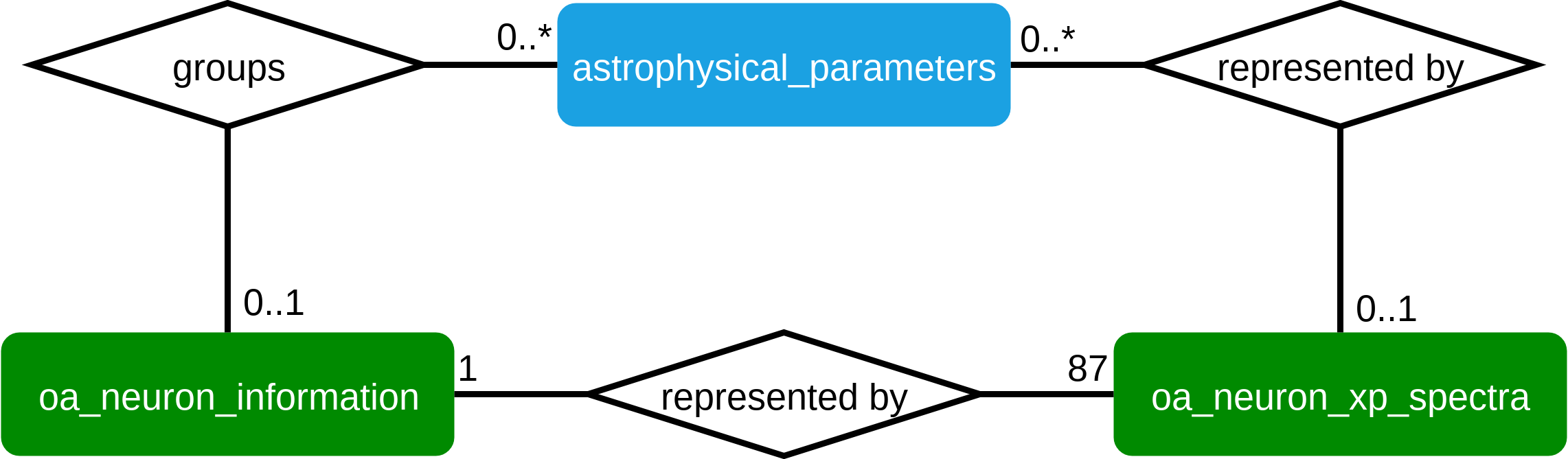
Figure 11.53: Relationship between all the tables in Gaia DR3 archive that contains OA products.

These products are essentially contained in three different tables of the archive, whose relationship can be observed in Figure 11.53, and contain the following information:

•

oa_neuron_information table contains non-multidimensional parameters related to the neurons, where each neuron is identified by an unique neuron_id, as well as two indices that allow to locate their position within the map (neuron_row_index and neuron_column_index). Basically, this table provides some statistics for each one of the neurons according to the objects that populate them. In particular, it contains mean, standard deviation, maximum and minimum values for different Gaia observables: $G$ (phot_g_mean_mag), $G_{\rm BP}$ (phot_bp_mean_mag), $G_{\rm RP}$ (phot_rp_mean_mag), proper motions (pmra, and pmdec), parallax (parallax), galactic latitude (b), number of transits in each photometric band (phot_bp_n_obs, and phot_rp_n_obs), astrometric parameter ruwe (ruwe) and excess colour (check Section 20.2.5 for further information about oa_neuron_information). It also contains some other relevant information, such as the number of sources populating a neuron (hits), the class label assigned to the neuron (class_label), if any, and the source_id of the centroid object (centroid_id). Finally, some quality indices based on the intra-neuron distance distribution are also provided: distance percentiles, $F W H M$ (distance_fwhm), skewness ( $S$ , distance_skew), kurtosis ( $K$ , distance_kurtosis) or the categorical index $Q C$ (quality_category).
•

oa_neuron_xp_spectra table contains multidimensional data related to XP spectrophotometry of the neurons, so that the preprocessed spectra for both prototypes (xp_spectrum_prototype_flux) and templates (if available, xp_spectrum_template_flux) for each neuron can be retrieved.
•

astrophysical_parameters table gathers information about the correspondence between the sources and the neurons, among other results produced by many different modules from Apsis. Regarding OA parameters, these are the actual neuron where a source lies (if it was processed by OA, neuron_oa_id), distance between the source XP spectra and the neuron prototype (neuron_oa_dist, and neuron_oa_dist_percentile_rank). Additionally, it also provides a processing flag (flags_oa).

Note that OA products are composed of many different parameters and just some of them were listed in this section. Further information about such fields can be found in Chapter 20. In addition, it must also be pointed out that the class_label parameter from the oa_neuron_information table was propagated to the extragalactic tables: qso_candidates and galaxy_candidates.

Finally, some use cases that can help the user to work with these tables can be found in Section 11.3.12, such as retrieving the sources assigned to a particular neuron, or to extract the prototypes or templates for the neurons. Furthermore, along with the Gaia DR3, a visualisation tool for SOM maps named “GUASOM flavour DR3” will be also released in order to explore OA products in an interactive and user-friendly manner. A detailed description of the tool and its features is provided in Álvarez et al. (2021).

Scope

As we mentioned in Section 11.3.12, the scope the of OA working package is to analyse classification outliers in Gaia DR3. Such module, as it was conceived, strongly depends on the performance of the general classification package DSC and its techniques (see Section 11.3.2).

In order to select outliers, OA relies on DSC combined probabilities, where all the sources that were assigned a probability of membership to any astronomical class above a certain threshold ( $\theta$ ) are rejected. For Gaia DR3, such a threshold was empirically adjusted to $\theta=0.999$ during the validation runs in Apsis, so that approximately 10% of the sources with a lower probability classification from DSC were processed. This means that, strictly speaking, more than classification outliers, OA is currently dealing with those objects that have lower probability classifications from DSC. Taking into account that most of the objects with weak classification probabilities have low brightness levels and are noisy objects, it can be expected that OA has to deal with the analysis and classification of low brightness stars and a sample of extragalactic objects. For those objects, we are providing an unsupervised classification that, in fact, is complementing the one proposed by DSC.

Following DPAC recommendations for Gaia DR3, the following filters were also implemented in order to discard some of the sources:

•

Remove sources with less than 5 transits or 241 measurements (for both BP and RP spectra).
•

Remove duplicated sources.
•

Accept only sources where AGIS converged to a solution.
•

Rejection list according to Gaia DR3 astrometric filters.

Results

For Gaia DR3, OA processed around 56 million objects among those with the lowest classification probabilities of membership to astronomical classes from DSC combined probabilities (see Section 11.3.2 for further details about DSC techniques). Therefore, it can be expected that these sources are, in general, low brightness stars and extragalactic objects, as it can be confirmed in Figure 11.54, which shows the distribution of mean magnitudes in the three Gaia bands for the neurons in OA SOM map.

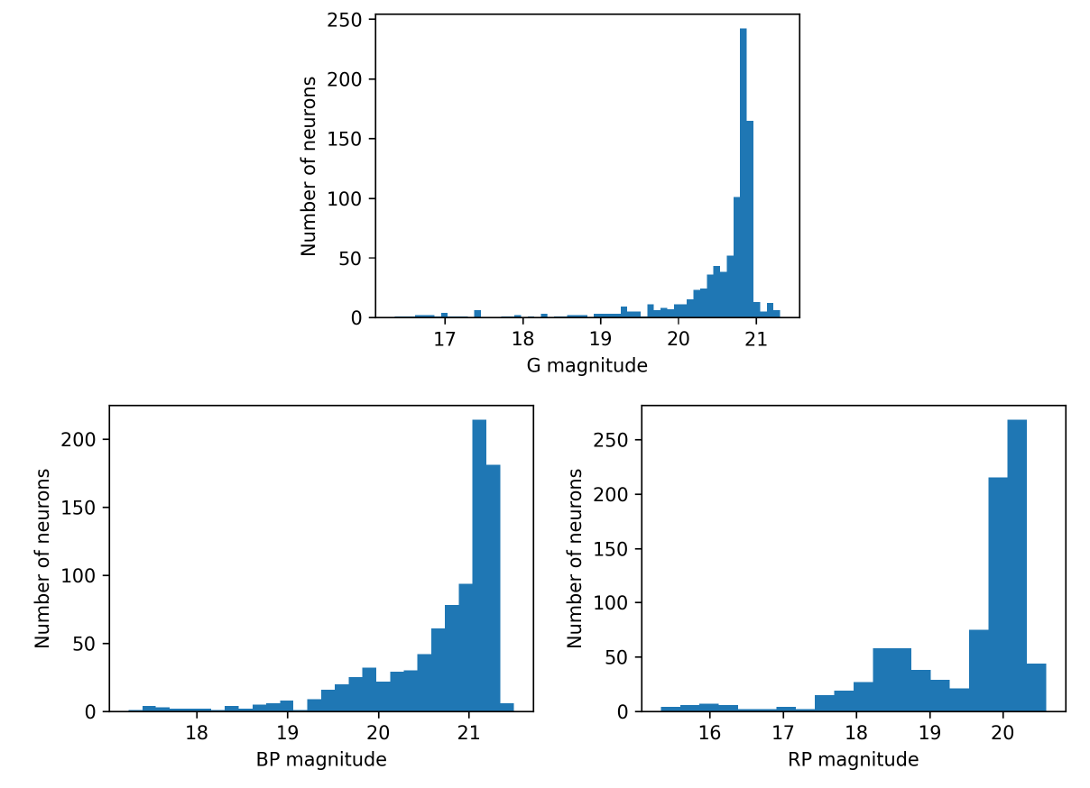
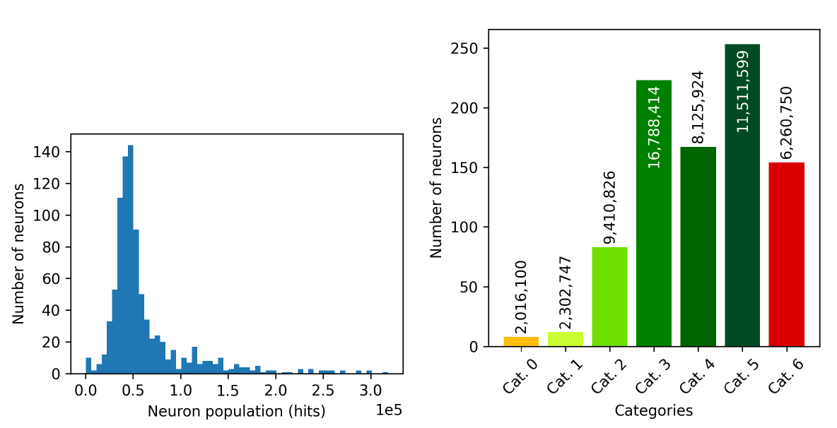
Figure 11.54: Neuron mean magnitude distributions for the three Gaia bands, where larger magnitudes are clearly predominant, as expected. (Upper) $G$ mean magnitude distribution. (Lower left) $G_{\rm BP}$ mean magnitude distribution. (Lower right) $G_{\rm RP}$ mean magnitude distribution.

Figure 11.55 analyses the number of objects populating the neurons. On the one hand, the left panel shows the histogram of neuron population (hits), with peaks around $50\,000$ objects, meaning that most of the neurons have an intermediate population, whereas a few neurons are very populated and allocate more than $100\,000$ sources or, in the same way, a very small number of objects are below such peak. On the other hand, the right panel shows the histogram of neuron quality categories, where the total number of sources belonging to such neurons is superimposed. As it can be observed, half of the neurons were assigned to a high quality category (HQN, high quality neurons, from category zero to three), whereas the rest can be considered low quality neurons (LQN, from category four to six).

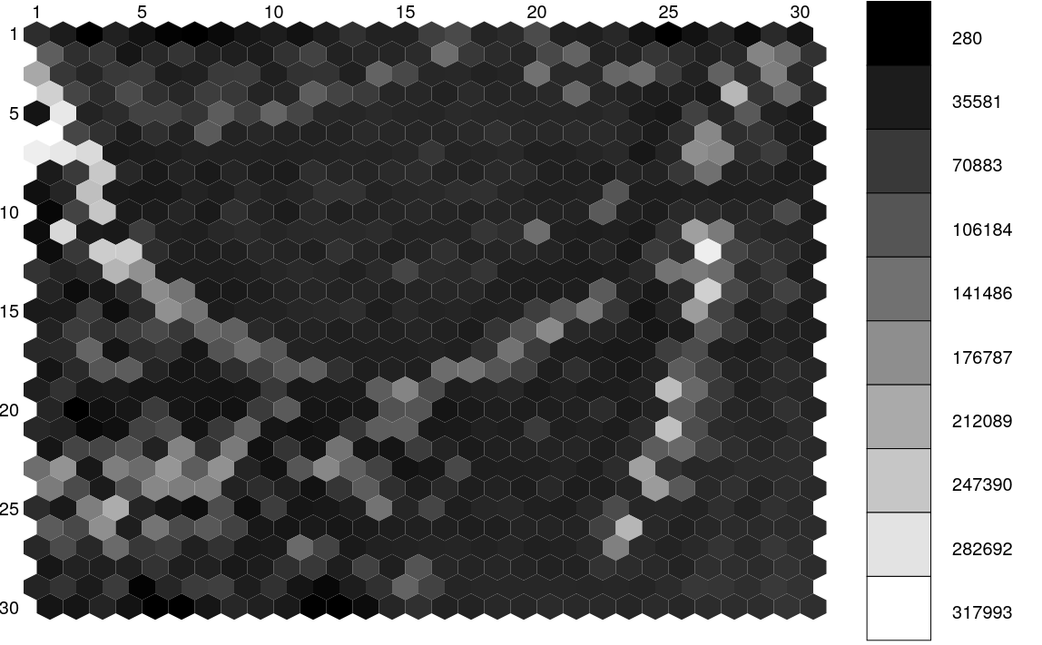
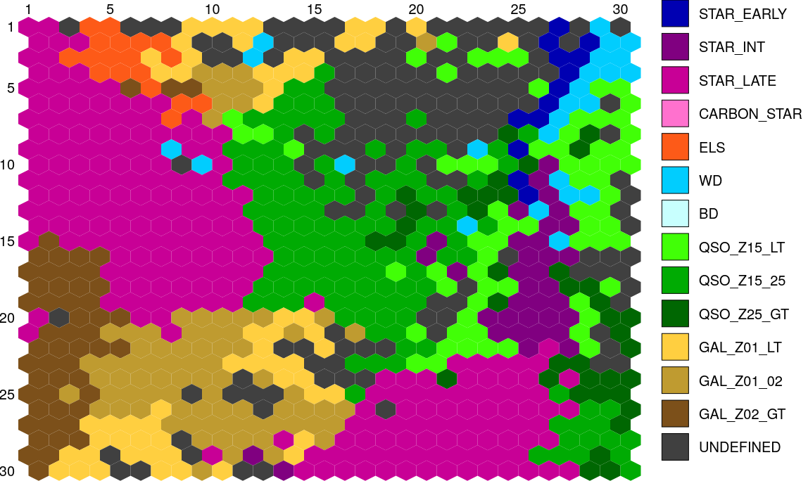
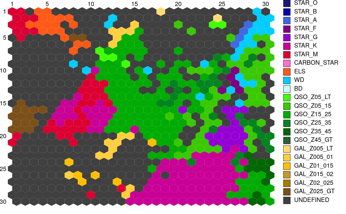
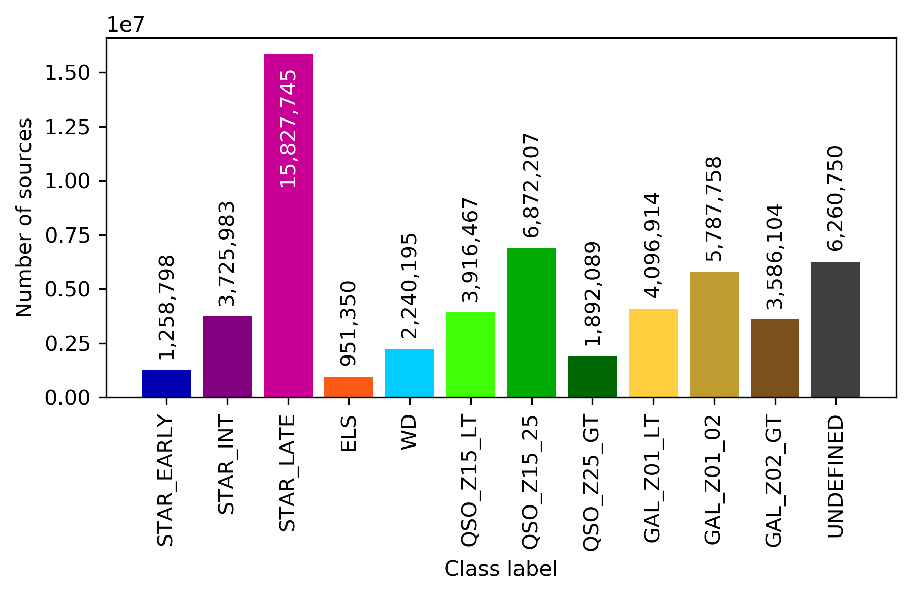
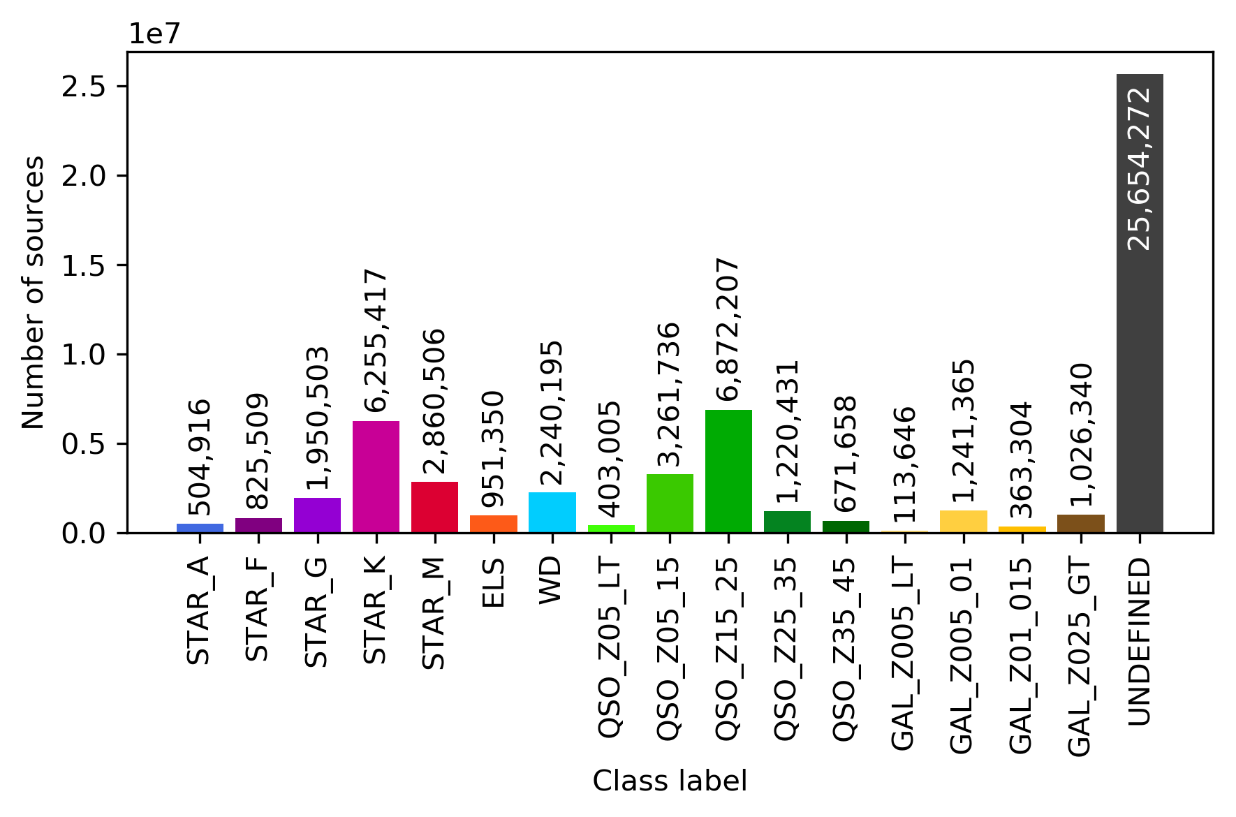
Figure 11.55: Neuron population analysis. (Left) Histogram that represents the distribution of neurons according to the number of objects that populate them, which is usually named as hits. (Right) Quality categories histogram, which shows the distribution of neurons per category, as well as the number of objects that populate such neurons (superimposed on the chart).

Similarly, Figure 11.56 displays the structure of the $30\times 30$ SOM map using GUASOM tool (Álvarez et al. 2021), where each cell represents a single neuron. The upper panel illustrates in grey scale the number of objects assigned to each neuron (hits), which allows to identify very populated areas. Additionally, the lower panel shows the distribution of quality categories within the map lattice, which reveals that high quality neurons (HQN) correspond to those neurons with the largest number of hits. This information is usually analysed together with the class labels assigned to each neuron (if suitable), which is displayed in Figure 11.57. Finally, Figure 11.58 shows the histogram for each one of the class labels that have been considered.

Figure 11.56: SOM map lattice visualised using GUASOM tool (Álvarez et al. 2021) to represent the population or hits of each neuron or cell through a greyscale (upper panel), and their quality category values (lower panel).

Figure 11.57: SOM map lattice visualised using GUASOM tool (Álvarez et al. 2021) to represent the basic class labels assigned to each neuron or cell (upper panel), and the specific class labels (lower panel). Note that all the neurons from quality category zero to five were labelled either with a specific (if suitable) or a basic class label. Those neurons that were not suitable for labelling remain as “undefined”.

Figure 11.58: Class label histograms for both types of class labels: basic (upper panel) and specific (lower panel). The height of the bars correspond to the number of sources that were assigned to such a label. “Undefined” means that no class label was found for a particular neuron.

Use

OA results can be used to perform a deep analysis of those sources that have lower probability classification from DSC, which mostly correspond to faint stars and extragalactic objects. To do this, OA provides many different parameters which were discussed in Section 11.3.12. In this section we cover some typical use cases that could be interesting for the final user when dealing with OA outputs:

•

The SOM map is composed of 900 different neurons and each one of them represents a group of similar objects, that may be candidates for an isolated study through the statistical parameters that are provided for each neuron or even through other different parameters available in the Gaia DR3 catalogue.
•

The prototype synthetic XP spectrum is provided for each one of the neurons, and it can be considered as a representative of the spectra for those sources that belong to a neuron. The template XP spectrum will be also available for those neurons that were assigned a class label.
•

For each neuron, different quality measurements or indices are available, so that a filtering can be performed by the final user in order to retrieve high quality neurons (HQN) or low quality neurons (LQN) and then perform a further analysis on the objects that belong to that specific group. In addition, the distance between the source XP spectra and the neuron prototype is also available in order to perform a finer filtering.
•

For the best quality neurons (from category zero to five), a hint on the astronomical class of the objects that populate such neurons will be provided through a class label, so that all the neurons or objects that are associated with a particular class can be identified and studied.

There are some known limitations when working with these results:

•

Currently, no templates were considered for binary stars, and therefore it may not be possible to deal with this type of objects within the OA outputs.
•

Some poor quality sources are assigned to the closest neuron in the SOM map according to the distance between the source XP spectra and the neuron prototype, but they may really provide such a poor fit that it renders useless their membership to that neuron at all. Therefore, we encourage the user to filter those sources using distance-based criteria as discussed above.

As we mentioned before, we specifically designed a client-server system (Álvarez et al. 2021) to facilitate the analysis work of SOM maps, that we named GUASOM (Gaia Utility for the Analysis of Self-Organising Maps). It was implemented with web technologies, to benefit from their flexibility and easy access to the information. The version of GUASOM that has been developed precisely for the spectra processed by the OA package for the DR3 is called GUASOM flavour DR3 and contains several visualization utilities that allow a user-friendly analysis of the information present on the map. The tool provides both classical and specific domain representations:

•

U matrix: This representation shows the distance among the different neuron prototypes, where less distance means more similarity. This is useful to identify groups of neurons populated by objects with similar SEDs. In our application the user can control the boundaries of the distance among neurons through a slider, with the objective of exploring the inner structure of the map.
•

Hits: It displays the number of objects for each neuron, allowing to identify dense regions in the map.
•

Parameter distribution: This visualisation shows the distribution of a particular parameter of the domain in the map, displaying the average values calculated in each neuron.
•

Catalogue labels: This graphic shows the representative label of each neuron according to a specific catalogue chosen by the user. The labels of the objects were obtained through the cross-matching procedure mentioned before. The user can control the qualified majority limit that the label has to reach to be representative through a slider.
•

Template labels: It is similar to the Catalogue labels visualisation, but in this case it is used the representative label of each cluster based on a template. It is selected the template that best fits with the prototype using the Euclidean Distance. One slider allows the user to control the distance between the prototype and its corresponding template in order to decide the adjustment threshold between them that allows assigning the label with sufficient confidence.
•

Category distribution: In this representation the distribution of a unique type of object is shown. The user can select the category to be displayed between a set of labels, according to the templates and catalogues available for the map. With this graphic the user can easily observe the regions of the map containing objects of the chosen type.
•

Colour distribution: It shows the colour distribution of the objects in the map, derived as the difference in magnitudes between two photometric bands, which correspond to the two photometers, BP and RP, and the colour is calculated as $G_{BP}-G_{RP}$ .
•

Novelty: This visualisation displays the distance between a selected template and its prototype. Less distance means less novelty because the template associated with the neuron is quite similar to the prototype, so it refers to a well-known object type. The user can select the set of templates to render.

The strength of the tool lies in its ability to explore the neurons and the objects assigned to them by means of the following specific representations:

•

Spectra: Represents the matched template, the object-centroid, and the prototype of a particular neuron. The user can also visualise the spectra of those objects in a neuron that best and worst fit the prototype.
•

Population: It shows the frequency of the different types of objects in the neuron according to the available templates or catalogues.
•

Statistical summary: The summary shows a table with the statistical information available for a neuron.

Some extra functionalities allow a complete interaction with other tools and databases:

•

Cross-match, where the user can select any source in a neuron, and perform a cross-match with a selection of external catalogues to retrieve the available information about the source.
•

Integration of SAMP (Simple Application Messaging Protocol), which is the most common protocol of the Virtual Observatory in Astrophysics, to communicate the visualisation with other astrophysical applications. The user can select several objects assigned to one or various neurons and send them to another tool using this protocol. Either the celestial coordinates or the spectra can be shared.

gaia data release 3 documentation