11.3.3 General Stellar Parametrizer from Photometry (GSP-Phot)
Author(s): René Andrae
Goal
GSP-Phot aims at a detailed characterisation of all single stars, only based on the low-resolution BP/RP spectra, apparent magnitude and parallax. (See Section 11.3.4 for GSP-Spec, which has the same task from RVS spectra instead of BP/RP spectra.) In particular, GSP-Phot estimates for each star its effective temperature , surface gravity , metallicity , radius , absolute magnitude in Gaia band and distance , as well as its line-of-sight extinction parameter and the derived extinctions in the Gaia bands , , (see Section 11.2.3), and the reddening .
Inputs
GSP-Phot primarily uses the internally calibrated BP/RP spectra that have been sampled by SMSgen (see Section 11.3.1). However, instead of the 120 pixels per BP and RP provided by SMSgen, GSP-Phot reduces both BP and RP spectra to only 50 pixels each by first adding up the integrated fluxes in any two neighbouring pixels and then discarding the five pixels on either end of the spectrum. GSP-Phot is one of the major consumer of computational power in the Apsis chain and GSP-Phot’s bottleneck is the fitting of the BP/RP spectrum. By reducing from 120 to 50 pixels per BP and RP, GSP-Phot is considerably reducing the overall computation time of Apsis. Furthermore, GSP-Phot makes use of the apparent magnitude and the parallax, see Section 11.2.1 and Section 11.2.2.
Further input data are model grids of synthetic BP/RP spectra for the four “libraries” named MARCS, PHOENIX, A and OB described in Section 11.2.3. GSP-Phot also makes use of an isochrone grid from PARSEC 1.2S Colibri S37 (Tang et al. 2014; Chen et al. 2015; Pastorelli et al. 2020, and references therein). That isochrone grid has a resolution of 0.01 in logarithmic age. In , the isochrone grid has a resolution of 0.03, ranging from -4.15 to +0.8.
Method
The main algorithm in GSP-Phot is Aeneas, which is an ensemble MCMC algorithm (Foreman-Mackey et al. 2013). The MCMC has four optimisation parameters, which are logarithmic age, initial mass, metallicity , and extinction (all other parameters are derived). Aeneas first takes the isochrone grid and uses 3D linear interpolation over logarithmic age, logarithmic mass and to obtain self-consistent temperature , surface gravity , radius and absolute magnitude . From the temperature, gravity, metallicity and extinction, Aeneas then uses 4D linear interpolation to obtain a model BP/RP spectrum (this is the computational bottleneck of GSP-Phot). This model BP/RP spectrum scales with (see Section 11.2.3). Therefore, Aeneas can perform an analytic weighted least squares fit to the observed BP/RP spectrum in order to obtain the amplitude of the model spectrum, from which the star’s distance can be obtained for given radius from the isochrone. This amplitude is then used to compute a from the BP/RP spectrum. The distance resulting from the BP/RP spectrum is also used to compute a second from the observed parallax. Finally, the distance obtained from the BP/RP spectrum’s amplitude, the absolute magnitude from the isochrone and the extinction (obtained from the same 4D linear interpolation as the BP/RP spectrum) are used to predict the apparent magnitude via . The difference between observed and predicted apparent magnitude provides a third , where the difference is weighted by where we introduced an error floor of 0.1mag in order to compensate for any imperfection in the isochrone’s absolute magnitude or the DR3 passband definition. The overall is the sum of the three contributions from the BP/RP spectrum, the parallax and apparent magnitude. As mentioned, the 4D linear interpolation over , , and not only produces an interpolated model BP/RP spectrum but also an interpolated extinction . Likewise, the extinctions and are interpolated in this way. This ensures that all extinctions are consistent with the underlying model SED and no transformation relations are needed, which might introduce additional systematic errors.
Concerning the priors used in the posterior probability maximised by the Aeneas MCMC, there are several in place: First, Aeneas uses a Hertzsprung-Russell diagram prior (Bailer-Jones 2011) which has been constructed from the Gaia Universe Model Snapshot (Robin et al. 2012). Second, over the allowed extinction range there is an ad-hoc extinction prior of exponential form, , where the mean value depends on Galactic latitude and distance ,
| (11.14) |
This specific functional form and the choice of coefficients is the result of several test runs. Lastly, there is a distance prior of the form , where the length scale depends on Galactic coordinates and has been mapped from the EDR3 mock catalogue of Rybizki et al. (2020). In an attempt to suppress outliers, the exponential length scale was further decreased by a factor of 10, which unfortunately caused GSP-Phot to systematically underestimate distances (see Figure 11.79). On top of that, the distance was further restricted to the range from 1pc to 100kpc. We emphasise that while these are formally correct priors, we do not use them in a strictly Bayesian context but rather as a regularisation in order to suppress spuriously large extinctions and distances.
The initial guess for the Aeneas MCMC is obtained in two steps: First, we employ extremely randomised trees (Geurts et al. 2006), which is a machine-learning algorithm that we trained on synthetic model spectra. Second, we follow up on the parameters resulting from ExtraTrees with a gradient descent algorithm called Ilium (Bailer-Jones 2010). The Aeneas MCMC starts either from the ExtraTrees parameters or the Ilium parameters, depending on which set of results achieves the higher posterior probability.
For every source, GSP-Phot is run separately for all four “libraries” MARCS, PHOENIX, A, OB. Consequently, there are, in principle, four sets of GSP-Phot results for every source (some results are removed during filtering as described below). All results are reported in the astrophysical_parameters_supp table such that users favouring certain libraries can always access those results. However, in the gaia_source and astrophysical_parameters tables, we also report the results for the “best” library. The best library is identified as the one having the highest mean log-posterior value averaged over the MCMC samples,
| (11.15) |
where denotes the GSP-Phot parameters, denotes the BP/RP spectra, the parallax, the apparent magnitude, and is the posterior probability of the -th MCMC sample (with a total of samples available). This choice was purely motivated by practical reasons, providing the best test results among other possible definitions (e.g. maximum posterior value, harmonic mean resulting in a Bayesian evidence). However, we emphasise that Equation 11.15 corresponds to a Monte-Carlo estimate of the differential entropy
| (11.16) |
i.e. . In other words, the best library is chosen to be the library whose posterior distribution has the lowest differential entropy, i.e. the best library provides the “most information” about the source from the point of view of information theory.
Outputs
The best-library results are available in the gaia_source and astrophysical_parameters tables and the separate results for MARCS, PHOENIX, A, OB (modulo filtering) are available in the astrophysical_parameters_supp table.
The provided parameters are effective temperature , surface gravity , metallicity , radius , absolute magnitude and distance , as well as its line-of-sight extinction parameter , the derived extinctions in the Gaia bands , , (see Section 11.2.3) and reddening .
For each parameter, the reported value is the median of the MCMC samples, while the reported lower and upper uncertainties represent the 16th and 84th percentiles of the MCMC samples. As additional quality controls, we also provide the MCMC acceptance rate and the mean log-posterior averaged over the MCMC samples.
Last but not least, we also provide the MCMC chains themselves, but only for a subset of sources due to the large data volume. Initially, MCMC chains have been provided for all best-library results. However, due to the filtering, some “best” results were removed and replaced by results from other libraries, which then come without MCMC chain. Concerning the MCMC chains, the full chain with 2000 samples is provided only for sources brighter than and for a random subset of 1% of sources fainter than . For all other sources, the provided MCMC chain is shortened to the last 100 samples in the final EMCEE ensemble state.
Scope
GSP-Phot has processed all sources down to with all four libraries (MARCS, PHOENIX, A, OB). This produced 2 251 091 833 results for 562 789 887 sources. However, not all of these results are of publishable quality. We filtered out the full set of results from all libraries for a source if one of the following criteria applied:
-
•
No parallax measurement was available.
-
•
The number of transits in the BP or RP spectrum was below 10 or 15, respectively.
-
•
For technical reasons, the whole source had to be removed, if one or more of the libraries failed to produce results. However, this happened rarely.
We filtered out results from individual libraries (keeping other libraries) for a source if one of the following criteria applied:
-
•
The MCMC acceptance rate was below 0.1, suggesting poor convergence.
-
•
The estimated distance differs from the measured parallax by more than ten times the parallax measurement error. We emphasise that this cut was performed on the parallax with zero-point correction used during CU8 processing (see Section 11.2.1). Therefore, the GSP-Phot distances may still deviate by more than ten sigma from the “raw” parallaxes published in Gaia DR3.
-
•
The predicted apparent magnitude differs by more than 0.1mag from the observed apparent magnitude.
If a best-library result was filtered out, it was replaced only by a “cooler” library. If the filtered best library was A, it could only be replaced by MARCS or PHOENIX but not by OB. Filtered best libraries from MARCS or PHOENIX, could only by replaced by PHOENIX or MARCS, respectively. Filtered best libraries from OB could be replaced by any other library.
After filtering, GSP-Phot still provides 1 665 152 313 results (73.97%) for 470 759 263 sources (83.65%). Of those sources, 449 297 716 still have MCMC chains. The remaining 21 461 547 sources without MCMC chains had their initial best library filtered out and replaced by another library.
Results
GSP-Phot results are generally good but there exist some caveats. Some main results will be highlighted here but we also recommend the user to consult the publications accompanying Gaia Data Release 3.
| catalogue | MedAD | MAD | RMSD | AD 75% | AD 90% |
| APOGEE DR16 | 169 | 418 | 1294 | 440 | 824 |
| GALAH DR3 | 110 | 150 | 228 | 198 | 315 |
| LAMOST DR4 | 110 | 156 | 253 | 198 | 327 |
| RAVE DR6 | 160 | 227 | 390 | 296 | 483 |
First, we compare the atmospheric parameters from GSP-Phot’s best library to literature values. Table 11.18 shows that the effective temperatures generally compare very well to literature values. Half of the sources differ from literature values by less than 110-170K (MedAD) for the various catalogues. For APOGEE in particular, the differences are typically larger than for the other catalogues because the APOGEE survey is probing regions of high extinctions (e.g. in the Galactic plane) where GSP-Phot suffers from the temperature-extinction degeneracy. The estimates compare particularly well to GALAH DR3 and LAMOST DR4, where 75% of sources differ by less than 200K and even 90% of sources differ by less than 330K. These results suggest that, at least in the low-extinction regime, GSP-Phot estimates are consistent with literature values to within typical uncertainties.
| catalogue | MedAD | MAD | RMSD | AD 75% | AD 90% |
| APOGEE DR16 | 0.218 | 0.406 | 0.626 | 0.570 | 1.054 |
| GALAH DR3 | 0.059 | 0.102 | 0.163 | 0.119 | 0.255 |
| LAMOST DR4 | 0.104 | 0.154 | 0.236 | 0.197 | 0.332 |
| RAVE DR6 | 0.252 | 0.335 | 0.465 | 0.451 | 0.709 |
Likewise, the GSP-Phot estimates also compare very well to literature values, as is summarised in Table 11.19. In particular, the agreement with GALAH DR3 is extremely good. Nevertheless, the comparison to APOGEE DR16 again stands out with much larger differences due to APOGEE probing high-extinction regimes where GSP-Phot is struggling with the temperature-extinction degeneracy.
| catalogue | MedAD | MAD | RMSD | AD 75% | AD 90% |
| APOGEE DR16 | 0.210 | 0.303 | 0.450 | 0.384 | 0.644 |
| GALAH DR3 | 0.210 | 0.238 | 0.295 | 0.326 | 0.452 |
| LAMOST DR4 | 0.204 | 0.248 | 0.330 | 0.328 | 0.477 |
| RAVE DR6 | 0.198 | 0.254 | 0.350 | 0.344 | 0.524 |
Table 11.20 compares GSP-Phot estimates to literature values. The differences are less than 0.21 for half the sources (MedAD) and below 0.4 for 75% of sources (AD 75%). However, as we shall see later in Figure 11.18a, there are strong systematic differences, which are not apparent from Table 11.20. In particular, there appears to be a generic underestimation of by 0.2, which may largely explain the median absolute difference of 0.21.
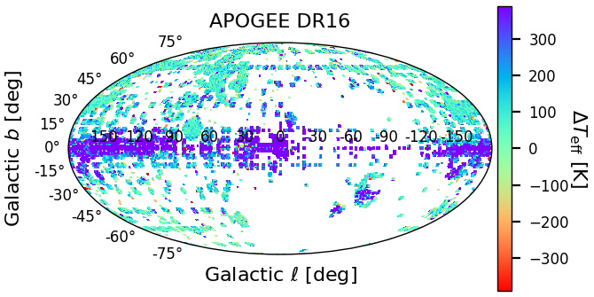
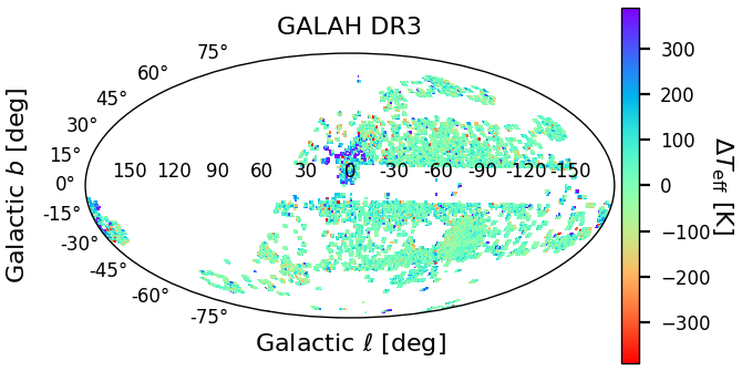
As is evident from Table 11.18, GSP-Phot temperatures compare better to surveys probing low-extinction regimes than to those probing high-extinction regimes. For representative examples for both cases, Figure 11.14 shows the differences w.r.t. literature values as skymaps for APOGEE DR16 (Jönsson et al. 2020) and GALAH DR3 (Buder et al. 2021). For GALAH DR3, the differences are mostly consistent with zero. However, for APOGEE DR16, the skymap shows clear evidence of GSP-Phot systematically overestimating in regions of high interstellar extinction. This is a consequence of the temperature-extinction degeneracy, which makes it difficult for GSP-Phot to distinguish between a low-extinction cool star and a high-extinction hot star from only the optical, low-resolution BP/RP spectra.
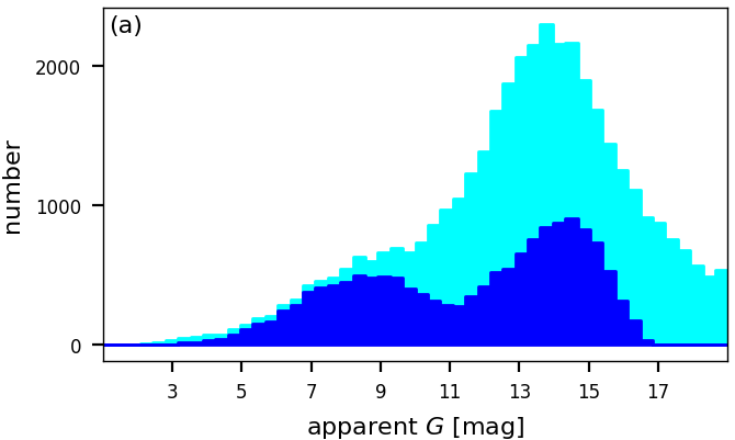
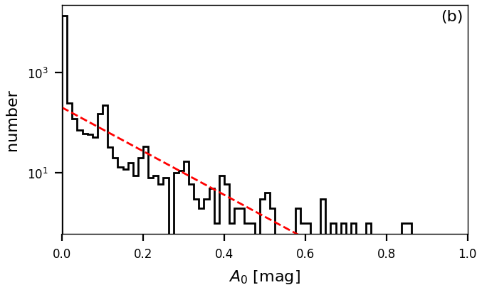
While the temperature-extinction degeneracy can be problematic in high-extinction regions, the GSP-Phot results are more robust in low-extinction regimes like the Local Bubble. Taking all Gaia sources with parallax larger than 20mas, we obtain a sample of 51,983 stars whereof only 14,862 stars have GSP-Phot results. While all stars have been processed by GSP-Phot, the filtering described before does remove many results. As is obvious from Figure 11.15a, the filtering does not affect all sources equally but instead, for nearby sources with mas mainly erases sources with apparent fainter than 10th magnitude. For such sources, the requirement that the GSP-Phot distance is within of the parallax measurement is failed by many sources. For the remaining 14,862 stars having GSP-Phot results, Figure 11.15b shows that the distribution of extinction estimates shows no drastic outliers and roughly follows an exponential. This is important since within GSP-Phot the fit parameter is not allowed to become negative and since the exponential is the maximum-entropy distribution of a non-negative quantity, Figure 11.15b suggests that the estimates in the Local Bubble are consistent with an intrinsic value of zero subject to random noise.
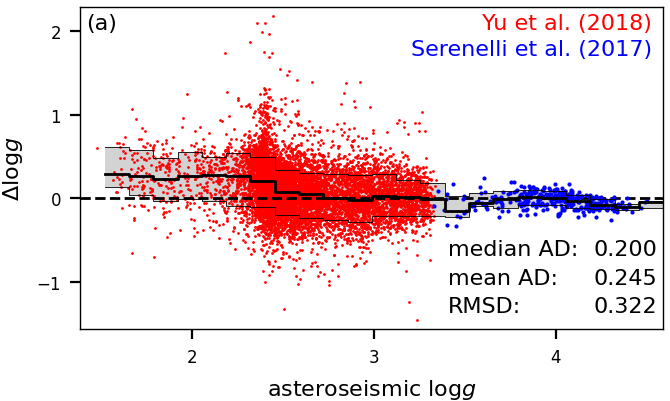
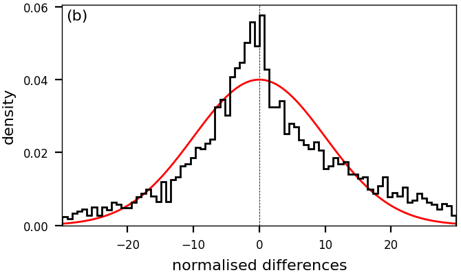
Despite the temperature-extinction degeneracy negatively affecting the and estimates, GSP-Phot does very well estimate the surface gravity of stars at least for stars brighter than . This is illustrated in Figure 11.16a, using a sample of stars with asteroseismic measurements for giant stars (Yu et al. 2018) and Main Sequence dwarfs (Serenelli et al. 2017). The overall agreement is excellent, with a median absolute difference of 0.2. This is a benefit of GSP-Phot predicting the apparent magnitude. There only is a minor overestimation of 0.2 of by GSP-Phot for giants with , but this bias is small enough such that GSP-Phot can still identify these stars as giants. Next, we exploit the fact that asteroseismic measurements have typical errors that are negligible compared to GSP-Phot’s own errors. This allows us to validate GSP-Phot’s uncertainty estimates by normalising the differences in estimates by GSP-Phot’s uncertainty. While there is no reason to assume that the distribution of normalised residuals should be Gaussian , Figure 11.16b demonstrates that GSP-Phot drastically underestimates the uncertainties for in this sample.
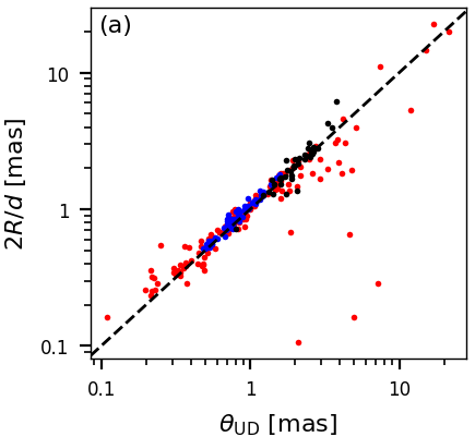
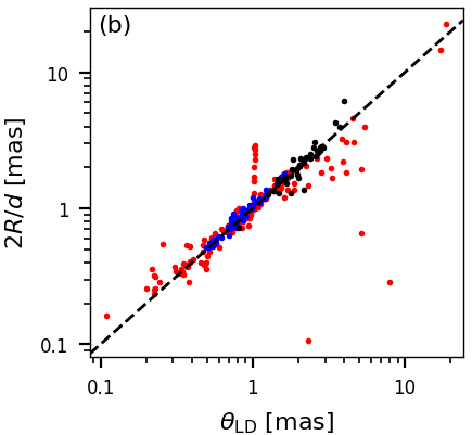
The radius and distance estimates, and , from GSP-Phot can be used to predict the angular diameter, . The results are compared to interferometric measurements from Boyajian et al. (2012a, b, 2013), Duvert (2016) and van Belle et al. (2021) in Figure 11.17. Even though there are a few outliers, the overall agreement across two orders of magnitudes is impressive.
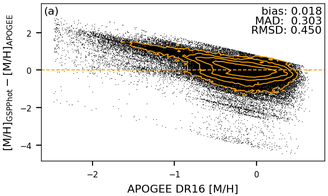
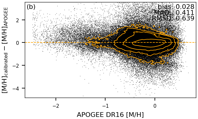
While is reasonably well constrained by GSP-Phot also fitting the apparent magnitude, the metallicity is really only directly constrained by the low-resolution BP/RP spectra. As a result, the GSP-Phot are of low quality and exhibit systematic errors. This is illustrated in Figure 11.18a, where we show the differences to APOGEE DR16 (Jönsson et al. 2020). First, there is a general underestimation of by 0.2. Furthermore, due to imperfect MCMC initialisation, GSP-Phot tends to favour solutions with solar-like metallicities, which causes the anti-diagonal trend in Figure 11.18a. However, GSP-Phot metallicity estimates should not be dismissed as useless because they can be empirically calibrated. To this end, we have trained a multivariate adaptive regression spline (Friedman 1991) to map from GSP-Phot results to metallicities from LAMOST DR6. Figure 11.18b demonstrates that this empirical calibration can remove the systematics for metallicities between -2 and +0.5, although it may increase the random scatter.
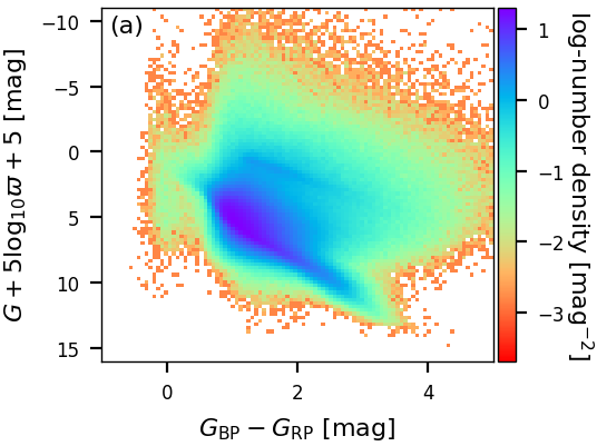
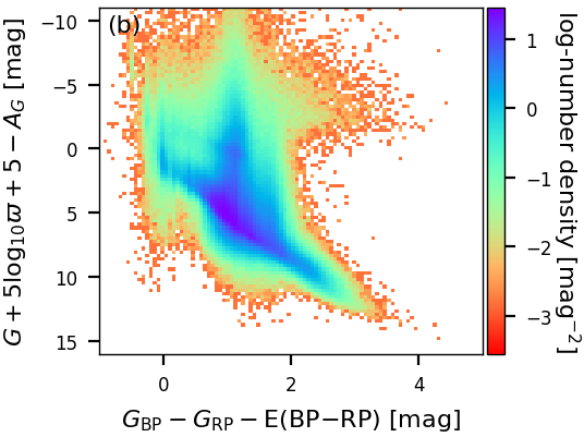
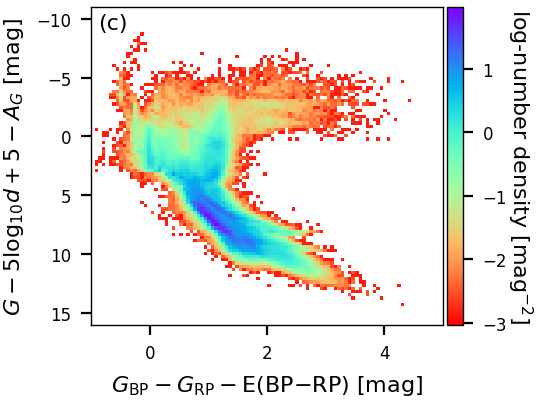
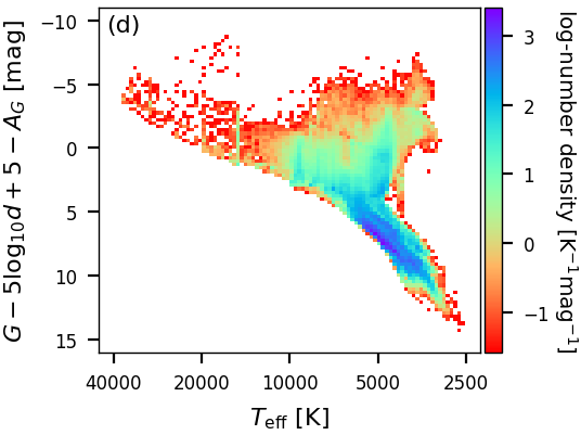
GSP-Phot results also allow to work with distributions of many sources. In Figure 11.19a and Figure 11.19b, we compare the observed coulour-magnitude diagram using only observables and the de-reddened colour-magnitude diagram using GSP-Phot extinction and reddening estimates. Although the de-reddening is not perfect and some artefacts remain, Figure 11.19b overall looks very good. One main source of scatter here are the parallax errors. Therefore, Figure 11.19c shows the de-reddened colour-magnitude diagram using the GSP-Phot distance estimate instead of the parallax. Evidently, there is much less noise here. As a side effect of less noise, more systematic effects become visible. In particular, Figure 11.19c fully benefits from GSP-Phot’s forward isochrone modelling insofar as unphysical parameter combinations cannot occur. The Hertzsprung-Russell diagram is shown in Figure 11.19d, which also looks very good and equally benefits from GSP-Phot’s forward isochrone modelling. Finally, we emphasise that neither Figure 11.19c nor Figure 11.19d show any white dwarfs. This is a consequence of GSP-Phot not using libraries of white-dwarf models and also excluding white-dwarf evolutionary states from the isochrone models. Therefore, GSP-Phot will treat white dwarfs as faint but otherwise normal stars and put them at large distances that are inconsistent with the white dwarf’s parallax measurement and thus they get filtered out.
Use
GSP-Phot results can be employed for a wide range of objectives starting from sample selection to direct analysis of individual stars. The user should keep in mind the following limitations and assumptions:
-
•
The results assume that a source is a single star and that this single star is not intrinsically variable.
-
•
For stars with low parallax quality () the GSP-Phot distances tend to be systematically underestimated due to on overly harsh distance prior. This particularly affects distant stars beyond 2 kpc. Nevertheless, for very good parallax measurements (), the GSP-Phot distances are reliable even out to 10 kpc.
-
•
Metallicity estimates from GSP-Phot are generally very poor, being 0.1 dex too low and exhibiting additional strong systematics. Therefore, we do not recommend to use the estimates from GSP-Phot. However, GSP-Phot estimates can be calibrated empirically, e.g. using LAMOST data.
-
•
The uncertainties are too small, i.e. differences to reference values are generally larger than accounted for by the GSP-Phot confidence levels.
-
•
Due to the temperature-extinction degeneracy, GSP-Phot results for stars with notable extinction (e.g. in the Galactic plane) tend to be unreliable. In particular, their effective temperatures and extinctions tend to be overestimated. Obviously, the use of near-infrared photometry would be very helpful to overcome this limitation, but the purpose of GSP-Phot is to provide results based on Gaia data only.
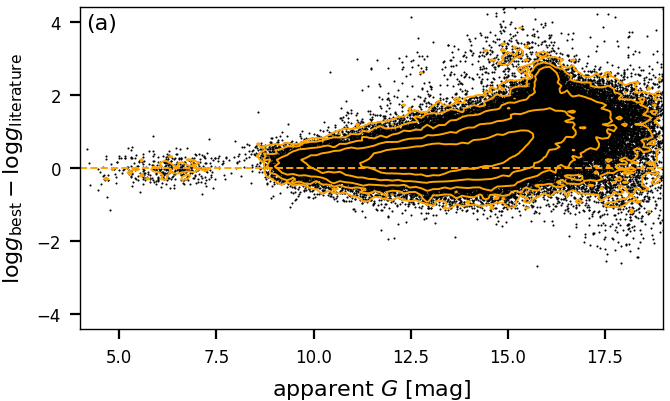
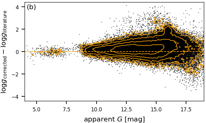
Figure 11.20: GSP-Phot estimate of compared to literature values from APOGEE DR16 (Jönsson et al. 2020) and GALAH DR3 (Buder et al. 2021) where the literature value is (i.e. excluding dwarfs). Panel (a) shows the best-library results. Panel (b) shows corrected values using Equation 11.17. Orange contours indicate source density dropping by factors of 3. -
•
For stars fainter than systematic errors appear, e.g. in surface gravity. This is evident from Figure 11.20. For RGB stars, the user may adopt the following simple model for the bias and use it to correct the GSP-Phot estimate of (e.g. for sample selections):
(11.17) This correction does not apply to Main-Sequence stars as those have been excluded from Figure 11.20. Instead, Main-Sequence stars may require a different correction. Other parameters such as may be affected by similar systematics towards the faint end.
In order to identify and remove outliers in GSP-Phot results, the user may explore the relative deviation in the predicted parallax as well as the deviation in predicted apparent magnitude . Both quantities have been used for filtering, restricting their ranges to and , respectively. Yet, the user may find that harsher cuts may be required in specific cases.
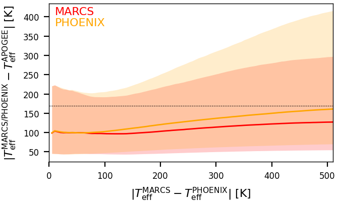
We explicitly encourage the user to deviate from our best-library recommendation whenever this appears useful. For example, studies of red-giant stars could ignore all results from our A and OB libraries and only use our MARCS or PHOENIX results for all sources. As a specific use-case, Figure 11.21 takes the sample of APOGEE DR16 (Jönsson et al. 2020) where GSP-Phot has problems with determining due to APOGEE probing regimes of high extinction and looks at the individual results for MARCS and PHOENIX. First, Figure 11.21 shows that both, MARCS and PHOENIX results, achieve overall median absolute differences below the 169 K achieved by the best-library results as reported in Table 11.18. Furthermore, Figure 11.21 shows that the more MARCS and PHOENIX results agree with each other, the more both of them also agree with APOGEE values. In particular, if we insist that MARCS and PHOENIX results agree to within 200 K, the absolute differences to APOGEE DR16 values are below 200 K for 75% of sources. In fact, Figure 11.21 suggests that the main impact of the temperature-extinction degeneracy and the outliers it is producing originate from erroneous best-library identification and that individual libraries may be much less affected by this. The downside of insisting on MARCS and PHOENIX to agree is that, due to the quality filtering of GSP-Phot results, only about one third of the stars in the APOGEE DR16 sample actually still have GSP-Phot results from both libraries.
From the given GSP-Phot results, the user can also estimate further derived parameters. For example, the user can compute the bolometric luminosity,
| (11.18) |
and the bolometric correction of the band,
| (11.19) |
While GSP-Phot does not directly provide absolute magnitudes in the BP or RP bands, GSP-Phot does estimate the distance and extinctions and . Therefore, the user can compute absolute BP or RP magnitudes using the observed apparent magnitudes via
| (11.20) |
Given those, the user can then compute bolometric corrections in those bands via
| (11.21) |
Likewise, the user can estimate apparent angular diameters of stars from the GSP-Phot estimates of radius and distance, or asteroseismic frequencies from scaling relations for solar-like oscillators. Uncertainties on those additional quantities can be obtained from the GSP-Phot MCMC samples by processing all samples through those equations and then computing, e.g., their median values and quantiles.
We point out that for all sources where an MCMC chain is available, the user can change the GSP-Phot priors using the method of importance sampling. For each sample, the MCMC chain provides the log-posterior and log-likelihood values, from which the user can recover our log-prior value:
| (11.22) |
In importance sampling, the user can then compute weighted expectation values of any function of GSP-Phot parameters provided in the MCMC samples
| (11.23) |
where the weights are given by the user’s new prior value divided by our old prior value:
| (11.24) |
We emphasise that the provided MCMC samples themselves do not change at all, but instead the difference is in the weighting introduced by importance sampling. Obviously, the user’s new prior must have some overlap with the GSP-Phot MCMC samples, otherwise all weights will be zero. As a simple example we consider the luminosity as a function of GSP-Phot temperature and radius:
| (11.25) |
For example, if we were to do this for known solar-like stars, we could then think of replacing the GSP-Phot prior with a new prior, say a Gaussian on centred around 5772K with a small width.