4.2.4 BAM data
Author(s): Lennart Lindegren
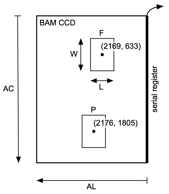
The Basic Angle Monitor (BAM) is a laser-interferometric device to measure variations of the basic angle on time scales from minutes to days. Line-of-sight variations are monitored by means of two interference patterns, one per field of view, projected on a dedicated CCD next to the sky mappers (Figure 1.2).
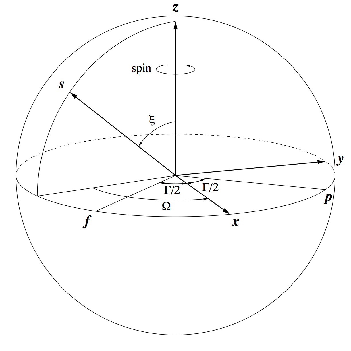
The BAM data show that the basic angle of the Gaia telescopes varies with an amplitude of about 1 mas and a period of 6 hours. The variations are very regular and phased with respect to the direction towards the Sun. For a constant solar aspect angle they are (mainly) a periodic function of the heliotropic spin phase (Figure 4.3). To first order, the basic angle variations can be described by a harmonic series in , with coefficients , that are only slowly varying with time:
| (4.82) |
Harmonic analysis has demonstrated the presence of harmonics up to at least order (45 min period). The highest detected harmonics have amplitudes of only a few . Superposed on this smooth variation are small discontinuities (jumps) and various other irregularities on short time scales. The purpose of the BAM data processing is to construct a numerical representation of the basic-angle variations, as measured by the BAM, to be used as input to the astrometric solution (AGIS). Two kinds of input are required:
-
1.
A list of detected basic angle jumps (times and amplitudes), and time intervals with irregular behaviour, that can be used to define breakpoints in the calibration model (Section 4.3.6).
-
2.
A spline fit of the basic angle variation as a function of time, including discontinuities, that can be used as a first-order basic angle corrector (BAC) in AGIS.
In AGIS the smaller jumps may be corrected by means of the spline, while for the larger ones there should be a break in the calibration model, since the jump amplitude measured by the BAM may not be representative for the whole astrometric field. By including all the jumps in the spline, the choice of break or no break is left to the user. It should be noted that additional variations of the basic angle and/or optical distortion, using VBAC and FOC, can be modelled on top of the spline derived from the BAM data as part of the global calibration model (Section 4.3.7).
Even though the basic angle corrections will in the end be represented by a spline, not using a harmonic series, there are good reasons to still use the harmonic model in Equation 4.82 as an intermediate representation. Firstly, the evolution of the harmonic coefficients is interesting in itself, in particular for better understanding the variations and possible correlations with other factors. Secondly, the harmonic model provides a convenient, accurate, and very robust interpolation for bridging minor gaps in the BAM data. The BAM data analysed until now cover data segments 0 through 6, i.e. from the start of the operational phase on 2014 July 25 until 2020 January 20 (OBMT 1078 to 9100 rev) or 66 months of data.
Generation
During normal operations of Gaia the dedicated BAM CCD is read out once every 23930 TDI periods or 23.518404 s. The CCD frame contains the interferograms (fringe patterns) from both fields of view (Figure 4.4), so the measurements are strictly simultaneous. The basic angle variations are deduced from the phase difference between the two fringe patterns in a single readout.
While the BAM data analysis for Gaia DR1 fitted an analytical model of the fringe pattern to the raw CCD data to derive the fringe phases, the analysis for Gaia DR2 and Gaia DR3 used a cross-correlation method. This is more precise (and possibly also more accurate) than the forward modelling approach, given that the observed fringe pattern deviates systematically from the somewhat simplistic analytical model used in the earlier analysis. Another improvement from Gaia DR1 is that the raw CCD data have been filtered for cosmic rays before the subsequent analysis, which drastically reduced the number of outliers in the fringe phases.
The cross-correlation method calculates the phase difference between two two-dimensional interferograms , by finding the maximum of the cross-correlation function
| (4.83) |
Direct summation is used, rather than the fast Fourier transform, since only a small range of displacements is needed for which the Fourier method gives no advantage. The displacement corresponding to the maximum of is obtained by fitting a cosine function
| (4.84) |
with , , , and as free parameters in an interval of pixels around the maximum (the fringe period is pixels). The fitted amplitude (), period (), and goodness-of-fit statistic provide useful diagnostics on the functioning of the BAM and for the further analysis.
The correlation method requires that the interferograms and to be compared are sufficiently similar, i.e. essentially in phase with each other over the whole image for the appropriate displacement . This prevents a direct cross-correlation between the interferograms at P and F in Figure 4.4: the different wavefront errors in the preceding (P) and following (F) fields make the fringe patters too dissimilar. For the same reason, the evolving wavefront errors may prevent cross-correlating interferograms obtained many days apart. For this reason, cross-correlation is only made between pairs of interferograms from the same field of view, and separated by at most 30 hr or five revolutions. The practical organization is depicted in Figure 4.5. One interferogram, indicated by the dot, is chosen as template for cross-correlating interferograms within a span of nine revolutions. The result is a time series of shifts relative to the template. To safeguard against the occasional bad template, ten different templates are used in a given span, producing ten different time series. A robust average (median) of the time series is computed after correcting each series for the offset produced by the different templates.

As indicated in Figure 4.5, successive spans are shifted by one revolution, resulting in average time series that typically overlap by eight revolutions. They are also shifted relative to each other due to the different templates used. The next step in the processing is to combine the overlapping time series into a single time series per field of view, giving the displacements of successive interferograms with respect to a common template. This is done by computing a weighted mean of the ten time series, after correcting for their offsets. A sliding cosine weighting function is employed to avoid introducing discontinuities at the endpoints of a span.
Short data gaps (less than a few revolutions) are readily bridged by the cross-correlations, provided there is no dramatic change to the instrument during the gap. Longer gaps cannot be bridged in this way, and the time series then has different zero points on either side of the gap. It is mandatory that the geometric calibration model has a breakpoint at such a time to compensate for the unknown offset in the BAM data before and after the gap. Table 4.2 lists the gaps in the BAM data for Gaia DR3 not bridged by the cross-correlations, which therefore require breakpoints in the calibration model.
| Gap length | Cause | ||
| 1320.998619 | 1329.999854 | 9.000 | decontamination #4 |
| 1338.998910 | 1339.999531 | 1.000 | |
| 2334.999097 | 2351.999937 | 17.000 | decontamination #5 |
| 4113.310238 | 4134.000545 | 20.690 | decontamination #6 |
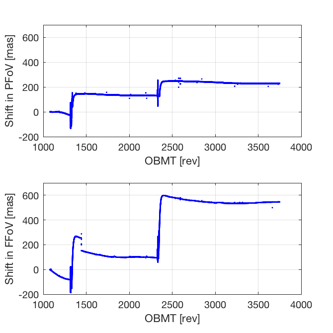
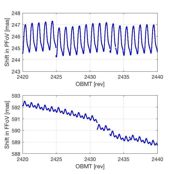
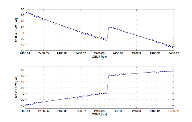
Figure 4.6 shows the fringe shifts derived for both fields of view. The two major disruptions caused by the contamination (around OBMT 1325 and 2340) are clearly seen. The large shifts after each decontamination, by a few hundred mas, are only apparent due the inability of the cross-correlation method to track the shifts across the large gaps. Figure 4.7 is a zoom on an arbitrary five-day interval, illustrating the various effects that need to be taken into account in the subsequent analysis: quasi-regular periodic variations, trends, and jumps. As shown by this example, when jumps occur they are not necessarily seen in both fields of view. It is therefore necessary to analyse the BAM data in each field of view separately, and only calculate the difference (which is the BAC) at the end.
The subsequent analysis of the BAM data needs the following inputs:
-
•
the time of each BAM measurement ();
-
•
the corresponding relative fringe displacements in the preceding and following fields, and ;
-
•
the goodness-of-fit measures (weighted RMS fitting errors), and ;
-
•
the heliotropic spin phase ;
-
•
the distance from the Sun to Gaia, .
The first three items are generated by the previously described cross-correlation processing. The times are corrected so that they refer to the mid-time of the CCD exposure. The fringe positions are converted from pixels to angular units by means of a nominal scale factor ().
The last two items require information from the attitude and barycentric ephemerides of the Sun and Gaia, and are computed as follows. Using GREM (Section 4.1.5), the distance to the Sun () at the time of the BAM measurement is obtained together with the observed (proper) direction to the Sun, . For the latter, GREM returns the rectangular coordinates in the Centre-of-Mass Reference System (CoMRS) , that is
| (4.85) |
The components of the same vector in the Scanning Reference System (SRS) ,
| (4.86) |
are obtained by the frame rotation (Equation 11 in Lindegren et al. 2012)
| (4.87) |
where is the quaternion representing the attitude of Gaia at the time of the BAM measurement. On the other hand, from Figure 4.3 it is seen that
| (4.88) |
from which and can be computed. (The angles and also appear in the definition of the scanning law of Gaia. However, while the scanning law is defined with respect to a non-physical object called ‘the nominal Sun’, the present angles represent the actual physical direction towards the Sun, that is the direction of the energy flux or Poynting vector. The physical and nominal directions may differ by up to about 01, which could matter for the description of the basic-angle variations. The angle defined through the equations above may be called the physical heliotropic phase angle in order to distinguish it from the corresponding nominal heliotropic phase angle used in the scanning law.)
The next step of the processing was a visual inspection of the shifts. The data are generally extremely clean, in the sense that there are very few isolated outliers, but already Figure 4.6 (especially the top panel) shows some features that look like outliers a few tens of mas above or below the main curve. Detailed inspection shows that these are typically groups of successive measurements lasting for several minutes which can nearly always be related to specific events such as station-keeping manoeuvres, configuration changes associated with calibration activities, or flux changes in the BAM data. Most probably they do not correspond to real basic angle variations, and they were therefore treated as gaps in the BAM data. Effectively, the fitted model was used to interpolate the shifts in these intervals.
Next, the jumps and a smooth variation of the fringe positions were simultaneously fitted over short intervals of time (typically one day). The generic model (here written for the preceding field, using superscript P) is
| (4.89) |
where , are continuous functions of time, represented by a cubic spline for and linear for , and are the times and amplitudes of the jumps. is a ramp function, increasing linearly from 0 to 1 for , where s is the CCD integration time for the BAM data. The width of the ramp sometimes makes it possible to determine the time of the jump to within a few seconds. For example, if the jump occurred exactly halfway through a CCD exposure, it would record a fringe position halfway between the positions recorded immediately before and after the jump. The fitted parameters are , , and the coefficients of and . Using harmonics was always found to be sufficient to represent the smooth, quasi-periodic variations.
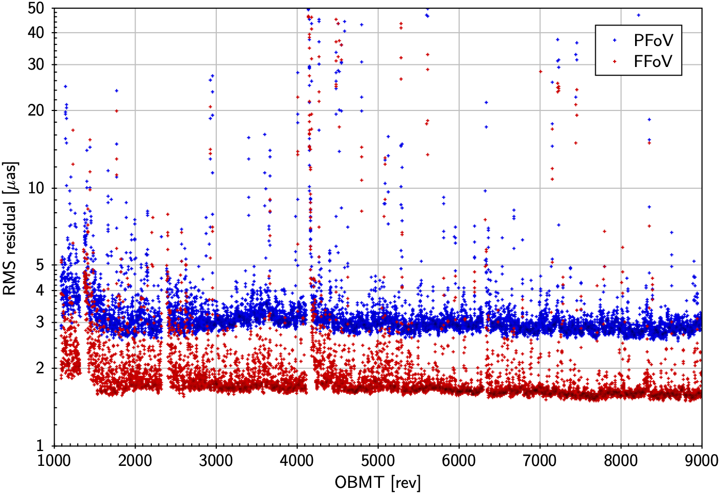
Figure 4.8 shows the temporal evolution of the RMS residuals from fitting Equation 4.89 to 4 rev intervals successively shifted by 1 rev. The median RMS value is 3.2 as in the preceding field and 1.9 as in the following. Enhanced RMS values are observed for some 200 rev (50 d) after the decontaminations.
The fitted model is strongly non-linear with respect to the times of the jumps, , and the number of jumps, . These are therefore estimated iteratively using a special procedure applied to the residuals of the previous fit, including the jumps detected up to that point. The procedure searches for the time where the tentative insertion of an additional jump would lead to the greatest improvement in the overall fit. If the amplitude of the tentative jump exceeds a fixed threshold, the jump is considered to be significant and added to the list of jumps. This is repeated on until no more significant jump are found. Figure 4.9 is an example of a jump fitted independently in both fields of view.
The Basic Angle Corrector (BAC) is a method that allows AGIS to compute an estimate of from the BAM data for arbitrary (expressed in TCB). The BAC will be used to correct the observations for the fast ( hr) variations of the basic angle, including jumps and the 6 hr harmonics. Additional corrections for the slow basic-angle variations, major jumps, and (optionally) the harmonics are introduced via the calibration model. The BAC will use a single spline to represent as a continuous function of time, with discontinuities at the times of detected jumps.
As a step towards constructing this spline, two time series are constructed representing and at equidistant times in OBMT, with additional points at the jumps. A time step of rev (168.75 s) in OBMT was chosen, which is small enough that a linear interpolation entails a negligible interpolation error (as). Since the same points in time are used for both time series, a similar time series for BAC is trivially computed as the difference between the two series.
Because the cross-correlation method cannot span interruptions much longer than a day, separate time series are constructed for the time intervals separated by such longer gaps (cf. Table 4.2). Five separate time series were therefore constructed for the OBMT intervals 1074.000–1321.000, 1340.000–2094.125, 2095.500–2179.125, 2191.000–2325.125, and 2352.000–3751.000. Using the jumps and harmonics determined from the previous analysis, the time series were computed by the following steps:
-
1.
The detected jumps and harmonics were subtracted from the cleaned BAM data. What is left is essentially a representation of in Equation 4.89 at quasi-regular times, but with a lot of gaps due to bad data intervals and outliers. It is not expected to have much high-frequency content apart from the noise, but it will contain all variations that cannot be represented by jumps or harmonics of order in . This includes, for example, any long-term trends and 24 hr variation of the BAM signals.
-
2.
The irregular time series resulting from step 1 was low-pass filtered using a running 31-point median filter. The result is a less noisy sequence defined on the same points in time as the unfiltered data.
-
3.
A regular sequence of OBMT was set up covering the required time interval. To this sequence, two more points were added at the time when a jump was detected in either field of view. For example, the first jump was detected in the following field at OBMT 1075.085222 rev. Therefore, the time sequence around this point looks like this in both fields: , 1075.0703125, 1075.0781250, 1075.0852220, 1075.0852220, 1075.0859375, 1075.0937500, .
-
4.
The irregular time series obtained in step 2 was linearly interpolated to the time sequence in step 3.
-
5.
The jumps and harmonics subtracted in step 1 were added back to the interpolated time series. For each jump, the two points at the same time give the result immediately before and after the jump. The jumps in the resulting time series are therefore instantaneous.
Contents
The output of the processing described in Section 4.2.4 consists of a cubic spline function fitted to the time series . A knot interval of about 10 minutes is sufficient to represent the harmonics (up to order ) to better than 0.1. Detected jumps are represented by four-fold knots inserted at the appropriate times. A list of detected jumps, , is also produced.
Usage in Gaia processing
The spline function representing the function , including discontinuities at the detected jumps, is used as a first-order correction of all astrometric measurements for the basic-angle variations. Additional corrections are computed in the astrometric solution as part of the geometric instrument model (Section 4.3.6) or global parameters (Section 4.3.7).
The list of detected jumps is used to select suitable breakpoints for the calibration model. Typically, jumps exceeding 0.1 mas in amplitude should result in a breakpoint. However, this is not always possible, e.g., if the resulting calibration interval would be too short.