14.5.1 Astrometry and Photometry
Three-dimensional KLD: Gaia DR3 vs Gaia DR2
Here we focus on comparing Gaia DR3 to Gaia DR2, in particular by computing the KLD in 2D for the whole Gaia DR3 and Gaia DR2, and the 3D KLD in small regions to explore spatial dependence on various photometric and astrometric quantities.
Summary of the results:
-
•
We find that the two and three-dimensional distributions are consistent between pairs of patches which are symmetric with respect to the scanning law.
-
•
When compared with Gaia DR2, we find Gaia DR3 to be systematically less clustered in subspaces containing positional information. We interpret this as an improvement on the systematics introduced by the scanning law.
Data used
The data used for the various tests performed is as follows:
-
•
2D KLD: We carry out a comparison of the gaia_source table, between Gaia DR3 & Gaia DR2. We do not apply any spatial selection, i.e., we consider the whole sky region altogether. For computing the KLD from (14.27), we consider limits that contain 99% of the data in each subspace, in order to exclude outliers.
-
•
2D KLD subsets: We also perform tests on two magnitude limited subsets of Gaia DR3. These are referred to as bt11: () and ft20: (). Again, we do not apply any spatial selection on these, and use the 99% limits to exclude outliers for our KLD calculation.
-
•
KLD patches: Finally, we perform our tests on four circular regions on the sky, labelled ‘patch-a’, ‘patch-b’, ‘patch-c’, and ‘patch-d’, each with a radius of 5 deg, and centred on () = (), (), () and () respectively. The regions contain stars on average. They are chosen such that ‘patch-a’ and ‘patch-d’ cover regions of high number of transits, while ‘patch-b’ and ‘patch-c’ have fewer transits. No filtering has been applied to the data, however, since Gaia DR3 has a larger range of magnitudes when compared to Gaia DR2, we apply a cut at phot_g_mean_mag .
Two dimensional KLD
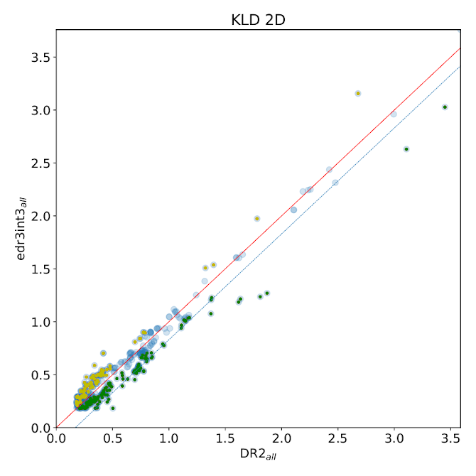
The first test compares KLD values between Gaia DR3 and Gaia DR2 for all 2D subspaces. This is shown in Figure 14.55. In the left panel, we plot the 1:1 comparison between the KLD in the two datasets. The sets for which there is a deviation greater than 10% with respect to Gaia DR2 are coloured yellow (higher) and green (lower) respectively. We notice that while a few subspaces lie very close to the 1:1 line, there is a large set of subspaces for which the KLD has dropped (green circles) in Gaia DR3. Furthermore, these sets in green follow a parallel track to the 1:1 line, with an offset of about 0.17. Noticeably, there are very few subspaces for which the KLD has increased considerably.
 |
 |
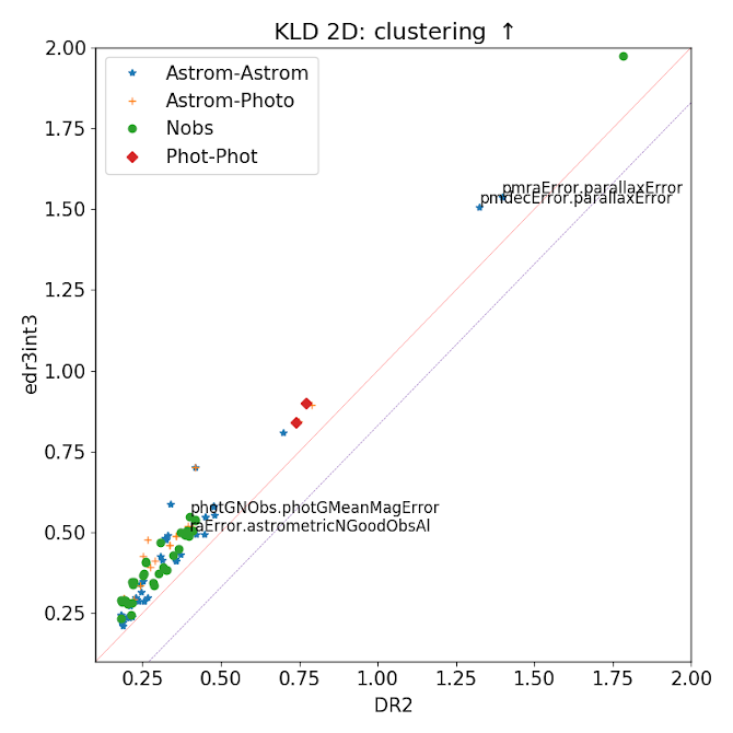
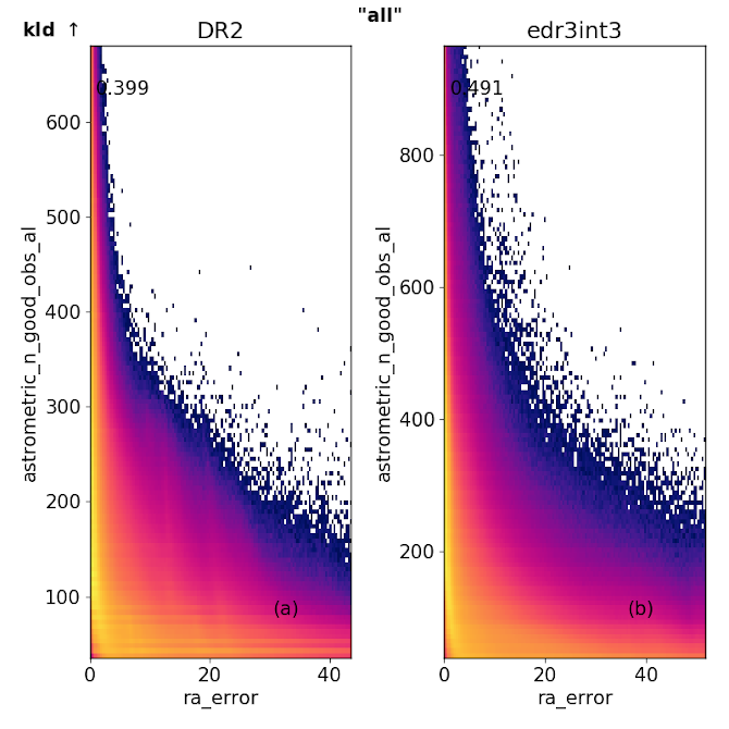
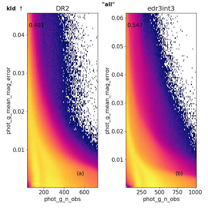
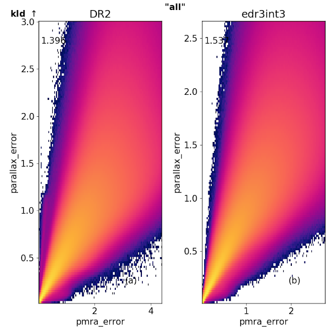
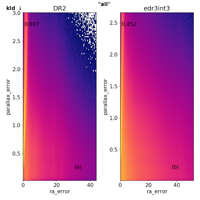
For the subspaces where the KLD has increased, we notice that many of these contain astrometric uncertainties such as errors in the observables ra, dec, pmra, pmdec and parallax. In Figure 14.57 we show the 2D histograms for select subspaces where the KLD has increased in Gaia DR3. We see, for example, that the ra_error and dec_error have high KLD in combination with observables relating to the number of observations (). This is not surprising, and can be interpreted as a consequence of increased observations resulting in lower errors in astrometry. Another improvement is noted in the higher KLD between parallax_error & pmra_error, shown in Figure 14.58. In this case, the range of the errors in both proper motion and parallax has dropped i.e., they point towards improved astrometry in Gaia DR3.
 |
 |
 |
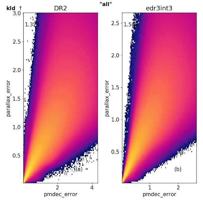 |
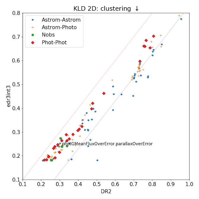
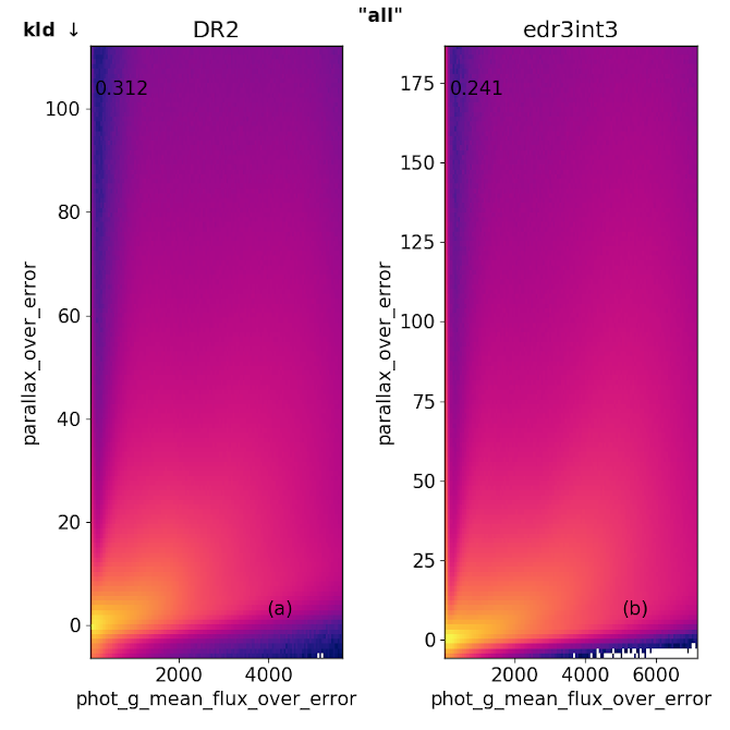
Conversely, in Figure 14.59, we show examples of where the KLD has dropped from Gaia DR2 to Gaia DR3. We note that the clustering between parallax_error and ra_error is lower. The range in both these errors is also smaller (especially for parallax_error). However, compared to Gaia DR2, the errors are less tightly correlated with each other, hence the lower clustering. In Gaia DR2, there are vertical striped patterns in the 2D distribution of this subspace, while in Gaia DR3, the distribution is smoother, and thus less clustered. Another example, is the comparison between parallax_over_error and phot_g_mean_flux_over_error. In this case, since the errors both in and magnitude, have dropped, the ranges for this subspace are much higher. As a result the KLD has dropped compared to Gaia DR2.
 |
 |
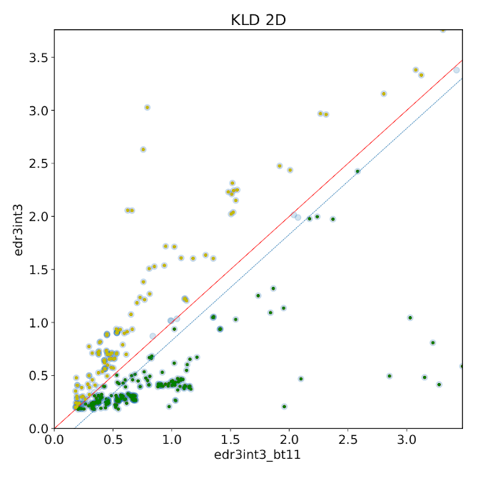
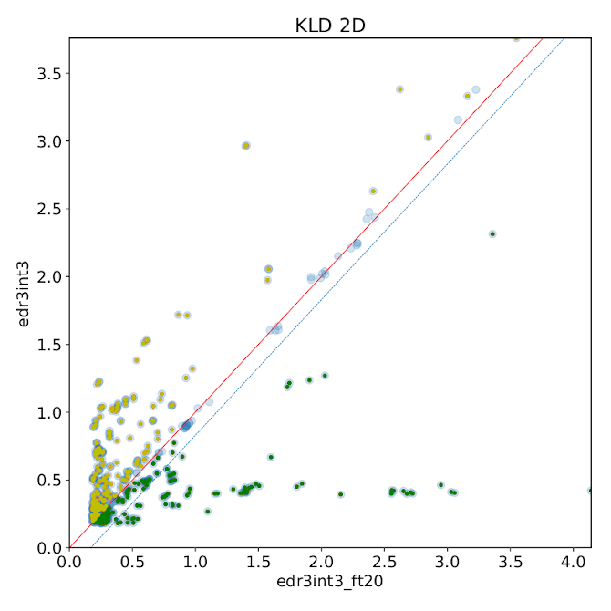
Comparison with subsets
We also compared the 2D clustering in Gaia DR3 with its subsets. In particular, we consider the brightest (bt11), and the faintest (ft20) subsets. Figure 14.60 shows that in general, compared to the all sky dataset, there is more clustering in the brightest subset, and less clustering in the faintest subset, except for quantiles in faint: the nearly horizontal distribution of points is due to the flux quantiles, which because of ‘noise’ on the measurements at the faint end becomes more uniform, and less on the 1-to-1 line.
While in the bright subset, where there is more clustering in the full dataset, this is because for the bright subset, most stars have really small errors and hence, all fall in one bin, making the KLD very low.
 |
 |
Three-dimensional KLD: Gaia DR3 vs Gaia DR2
The tests performed here are to assess if the astrometric and photometric data exhibits similar statistical properties, such as clustering and correlation between different observables on several small regions on the sky. The idea here is to test where any observables or a combination of observables exhibits unexpected properties on small scales. The tests are executed for all parameters in common between Gaia DR3 and Gaia DR2 as well as for a few selected parameter subsets.
We compute the 3D KLD using subspaces that contain combinations of ra, dec, and any other parameter. The goal is to assess how much position-dependent substructure (i.e. clustering) is present in the data. When computing the KLD statistic we use limits that contain 99% of the data in each subspace, i.e. we do not consider the top and bottom 0.5 % of the data points in each subspace to avoid outliers.
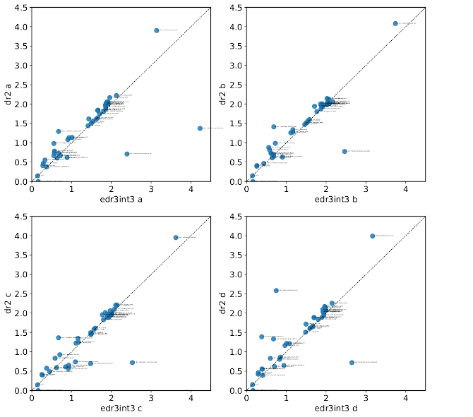
In Figure 14.61 we observe the 3D KLD values for ‘patch-b’ and ‘patch-c’ to be in good agreement. Since these patches are symmetric w.r.t. the Galactic centre and plane, this is the expected behaviour. A similar behaviour is observed for the other patch pair.
Overall, we observe that parameters related to astrometric precision (e.g. pmra_error), tend to be more clustered (higher KLD value) in Gaia DR2 than in Gaia DR3. Even though we do not consider the top and bottom 0.5% of the data while computing the KLD, some outliers may still remain, resulting abnormally small KLD values. We find that the subspaces containing astrometric_excess_noise_sig and phot_g_mean_flux_error suffer from this effect.
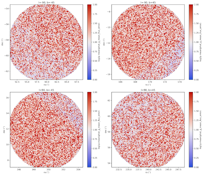
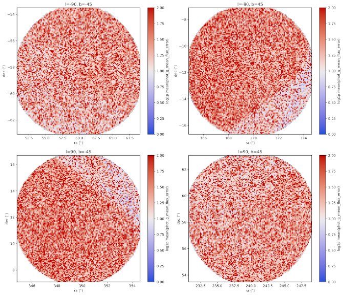
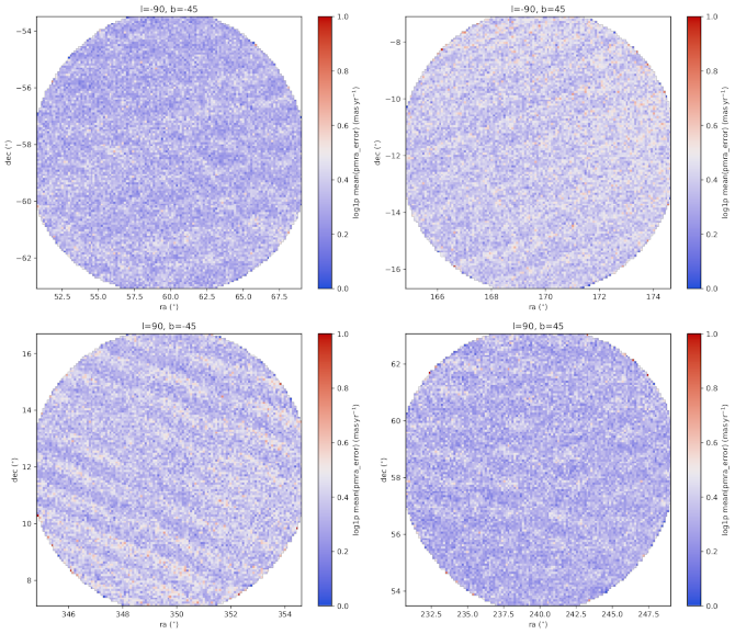
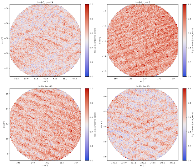
To exemplify the differences observed in the KLD values, we compared the on-sky distribution of two average quantities that appear to be less clustered (lower KLD value) in Gaia DR3 than in Gaia DR2. In Figure 14.62 we show the on-sky distribution of the average phot_g_mean_flux_error. We notice that this photometric quality quantity has improved in the sense of being more uniform as well as having a lower average value, when compared to Gaia DR2. We attribute this to the higher number of visits. In Figure 14.63 we show the same but the averaged quantity here is pmra_error. This quantity shows the characteristic scanning-law pattern systematics, which is evident on smaller scales than the previous figure. We attribute this to the sensitivity of astrometric parameters to the orientation of the visits, and not only their amount.
 |
 |
 |
 |